Quantcast
Channel: SCN : Blog List - SAP HANA Developer Center
Viewing all 676 articles
Browse latest View live

Building an Analytic & Calculation View from the Wikipedia HANA tables for use with SAP Lumira

$
0
0

Welcome to part 5 in this series of demonstrating how to analyze Wikipedia page hit data using Hadoop with SAP HANA One and Hive. In part four “Enhancing the Wikipedia data model using fact and dimension tables with SAP HANA”, I will use SAP HANA Studio to create an Analytic & Calculation view based on the PAGEHITSFACTTABLE fact table and the three dimension tables:  DIMPROJECT, DIMLANGUAGE and _SYS_BI.M_TIME_DIMENSION. I will also cover the initial step of granting SELECT permissions to the _SYS_REPO user for the SCHEMA that that holds the fact and dimension tables so that you can actually save your Analytic View. I will be covering the high-level components shown in the diagram below.

01 Diagram.png                   

Let’s get started!


Launch SAP HANA Studio. If not connected to database, click on the Choose Connection button on top right. Select your HANA database instance and click OK.


Make sure that the _SYS_REPO user has SELECT permissions to the WIKIDATA schema

For first time users of the data modeler in SAP HANA Studio, you must grant SELECT permissions to the internal _SYS_REPO user so that the data modeler can access the tables in your schema. If you forget to do this step, the data modeler cannot save the Analytic View.

In the SAP HANA Systems Pane on the left, expand by clicking on the arrows next to the following in order: HDB (SYSTEM) -> Security -> Users. Then, double click on ‘_SYS_REPO’ under Users. This displays the permissions page of the _SYS_REPO user as shown below.

02 User access.png 

Switch to tab SQL Privileges as shown below and click on the Plus button just above the list of SQL Objects to add the new permission.

03 SQL Privs.png 

Under Type name to find a catalog object, enter ‘WIKIDATA’. Select the WIKIDATA schema and click OK.

04 select schema.png 

Under SQL object, select WIKIDATA. In the Privileges for 'WIKIDATA' window on right, check SELECT and select Yes for Grantable to Others.

05 add select privs.png 

Close the document *HDB-_SYS_REPO by clicking on the X in the tab and click Yes when prompted to save changes.

06 save privs.png 

Data modeling using the Modeler perspective

In order to access the tools to create an Analytic Package and Analytic View within the package, you need to open up the Modeler perspective.

In the top menu, click on Window, go to Open Perspective and click on Modeler. If you do not see Modeler, select Other and click on Modeler followed by OK.

07 Open modeler.png 


HANA Studio should display the Quick Launch page. If you do not see it, go to the Help menu and select the Quick Launch command.


Create an Analytic Package

The first step to exposing data to SAP Lumira is to create an Analytic Package. The Quick Launch page makes it obvious by displaying the first step in the middle of the Quick Launch page. Just click on the Create… button to get started.

In the Quick Launch tab, Welcome to Modeler window, select Package under New if it is not already selected and click on the Create… button.

08 Quick create package.png 

I will call this package WIKICOUNTS and add a description as shown below. Click OK, when you are ready to continue.

09 new package.png 

NOTE: I am taking a short cut here by leaving the Person Responsible value as SYSTEM. In real life, you should use a lower privileged user account.


Create an Analytic view with the fact table and the three dimension tables

SAP Lumira uses the Analytic View as a first class data source, so it is time to create one. In the Quick Launch tab, select Analytic View under New and click on the Create… button.

10 create analytic view.png 

In the New Information View pop-up, enter the name for information view and description as shown below.

11 define view.png 

We now have to associate the container Package with The Analytic View. To do that, click on Browse… next to the package field, select the WIKICOUNTS package and click OK.

12 select package.png 

Click on Finish to complete the naming of the view and continue on to the designer.

I now need to add the four tables that will be part of the Analytic View. To do that, I need to use the Data Foundation block in the Scenario pane. Just click on the Data Foundation in the Scenario pane and the click on the + sign that appears next to it to display the Find dialog.13 data foundation.png

I now need to find each table and select in for the data mode. Just type in the name of the table, in this case I start with PAGE to display all the objects that start with PAGE and then select the PAGEHITSFACTTABLE and click OK to add it.

14 find table.png 

I then followed the same process for the _SYS_BI.M_TIME_DIMENSION, WIKIDATA.DIMPROJECT and WIKIDATA.DIMLANGUAGE tables. Here is what the screen looks like after adding the tables.

15 tables added.png 

Place the fact table – PAGEHITSFACTTABLE in the middle of the schema by selecting it and dragging it. This will make it easier for creating relationships.

16 arrange tables.png 

Creating relationships within the Analytic View

I now have to create the relationships for the Analytic view. The idea is to join the lookup column in the dimension table to the corresponding column in the fact table. To setup the relationship between the M_TIME_DIMENSION and PAGEHITSFACTTABLE table, I first select the DATE_SAP column in the M_TIME_DIMENSION table and then drag a relationship line to the EVENTDATE column in the PAGEHITSFACTTABLE table. The order you do this operation in is important so that you get the correct one to many (1..n) mapping. That is, drag the column from the dimension table to the lookup column in the fact table.

17 create relation.png 

Notice how the Properties dialog shows the properties for the relationship. To create the other two relationships, do the following:

  • Drag the LanguageCode column from the DIMLANGUAGE table to the LANGCODE column in the PAGEHITSFACTTABLE table.
  • Drag the ProjectCode column from the DIMPROJECT table to the PROJCODE column in the PAGEHITSFACTTABLE table.

18 relation creation complete.png 

I rearranged the tables to come up with something that makes the diagram look like a “star schema” as shown above.


The next step is to add the columns from the fact table and dimension tables as output columns. I am going to add them in a specific order to note the logical hierarchy of the data as follows:

  • Right click on ProjectTitle in the DIMPROJECT table and select the Add to Output command. I do not need to add PROJCODE from the PAGEHITSFACTTABLE table because the join will correctly hook up the correct value for the ProjectTitle.
  • Right click on Language in the DIMLANGUAGE table and select the Add to Output command.
  • Click on PAGENAME in PAGEHITSFACTTABLE and press Shift+Click on Hour to multi-select PAGENAME, YEAR, MONTH, DAY and HOUR columns. Then, right click on the selected range and choose the Add to Output command.
  • Select both the ENGLISH_DAY_OF_WEEK and ENGLISH_MONTH columns in the M_TIME_DIMENSION table. Then, right click on the selected range and choose the Add to Output command.
  • Finally, select both the PAGEHOTCOUNTFORHOUR and BYTESPERHOUR columns in the PAGEHITSFACTTABLE table. Then, right click on the selected range and choose the Add to Output command.

Your diagram and list of output columns should look like the screen shot below.

19 attributes added.png 

Next, I have to specify the actual measure columns as follows:

  1. Click on the Semantics object in the Scenario pane to display the Details for the view.
  2. Scroll down the list of Local Columns, select the PAGEHITCOUNTFORHOUR column.
  3. Press the Mark for Measure command just above the Label Column as shown in the screen below.

20 mark for measure.png 

HANA Studio automatically determines the rest of the attributes and measures during the Save and Validate step.

The last two steps are to perform the Save and Validate command followed by the Save and Activate command. Just click on each of these commands shown in the tool bar below to deploy the view.

21 deploy view.png

As you can see in the Job Log above, the model was validated and activated as expected. The Model Validation displays a Status of Completed with warnings. To see what those warnings are, just double click on the message to view the Job Details.

22 job warnings.png

Since I am not doing anything with ABAP or the BI Virtual InfoProvider, I can ignore the warnings. Click OK to close the dialog.


I can now do a quick test to view the data by clicking on the Data Preview command as shown below.

23 data preview.png

Next, I will drag the ProjectTitle column into the Labels axis and the PAGEHITCOUNTFORHOUR column into the Values axis to display a validation of the data lookups as shown below.

24 hits by project.png

Creating calculated columns using a Calculation View

I want to make two more enhancements to the data model. First, I want to create a calculated measure that computes the BYTESPERHOUR divided by PAGEHITCOUNTFORHOUR to see how pages can grow over time for current event topics. Second, I want to add a hierarchy for the page hit date so that I can see data by year, month, day and hour easily within SAP Lumira.


To do these changes, I need to create a Calculation view that takes the PAGEHITS Analytical View as an input and then adds the enhancements.


To get started, navigate to the WIKICOUNTS package and then right-click and choose the New> Calculation View… as shown below.

25 create calc view.png

In the New Calculation View, I will enter in the name of the view PAGEHITCALCVIEW, provide a meaningful description and then click Finish.

26 name view.png

You should now see the Calculation View design surface that looks like the screen below.

27 calc view surface.png

Next, I will

  1. Select the PAGEHITS Analytic View in the object explorer
  2. Drag the PAGEHITS Analytic View under the Output object in the left pane for the designer.
  3. Drag a connection line from the PAGEHITS view to the Output object.
  4. Click on the Output object to start enhancing the model.

28 connect view to output.png

Creating a Calculated Measure

To create the Calculated Measure to compute the average size of the page for a given hour, I need to add the PAGEHOTCOUNTFORHOUR and BYTESPERHOUR columns as measures. I will right click on each of the columns and select the Add as Measure command. You should see the two columns under the measures folder. This makes the measures available for the next step.

29 add measures.png

I will now right click on the Calculated Measures folder in the right hand output pane and select the New… command to display the Calculated Measures dialog. I will give the measure a name and description as shown below.

30 define calc.png

To build the expression in the Expression Editor, I did the following:

  1. Expanded the Measures under the Elements list
  2. Double clicked on the BYTESPERHOUR measure
  3. Double clicked on the divide by symbol “/
  4. Double clicked on the PAGEHITCOUNTFORHOUR measure
  5. Clicked on Validate to verify the expression and click OK to clear the validation message box
  6. Clicked OK to complete the measure definition.


Creating a hierarchy based on date attributes

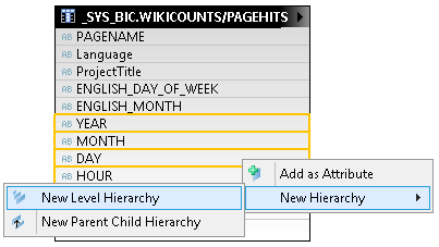
I could add the year, month, day and hour attributes as individual attributes, however tools like SAP Lumira can additional filtering and shaping of results when using a date based hierarchy. Building a date-based hierarchy is simple. To do so, I Shiftselect the YEAR, MONTH, DAY and HOUR attributes and the right click on them and choose the New Hierarchy> New Level Hierarchy command as shown below.

http://i1114.photobucket.com/albums/k540/billramo/31newhierarchy.png

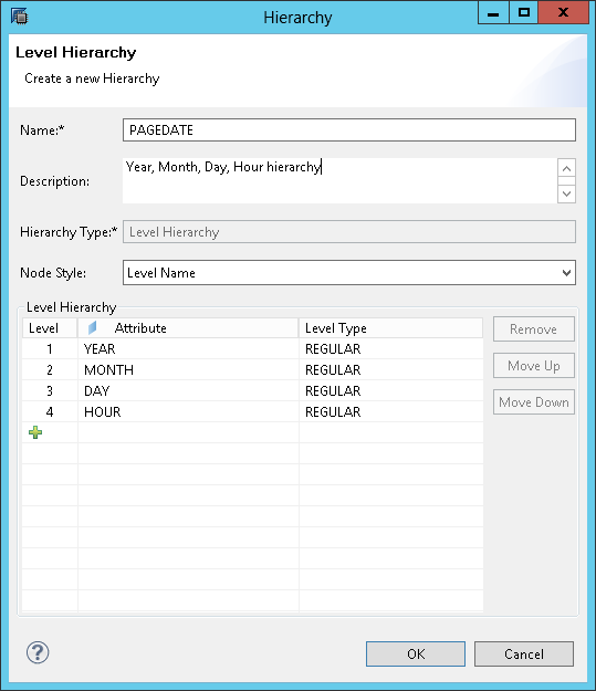
I can then fill in the name and description fields as shown below to complete the operation. This is because the order of the fields do not need reorganization.

http://i1114.photobucket.com/albums/k540/billramo/32namehierarchy.png

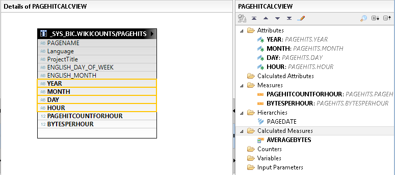
Clicking OK completes the operation. Notice that when I added the hierarchy, HANA Studio added the individual date attributes under the Attributes folder.

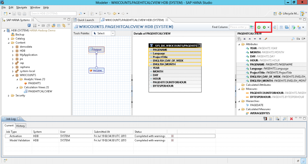
http://i1114.photobucket.com/albums/k540/billramo/33hierarchyadded.png

Adding the rest of the attributes to the output

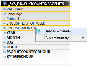
The only thing left to do now is to add the rest of the attributes to the output. To do this, I just need to Shift select the remaining columns, right click and select the Add as Attribute command.

http://i1114.photobucket.com/albums/k540/billramo/34addattributes.png

That is it! I can now run the Save and Validate command followed by the Save and Activate command to complete the creation of the Calculation View.

http://i1114.photobucket.com/albums/k540/billramo/35deploycalcview.png

At this point, I cannot wait to jump into SAP Lumira to see that mysteries I can uncover from the Wikipedia data. In the next blog, I will show you how to use SAP Lumira to analyze data using the Calculation View I just created.


Just to wrap up, you should have a good appreciation of how to do the following:

  • Grant rights to the _SYS_REPO user to the schemas used for the views
  • Using the Modeler perspective and the Quick Launch page for performing actions
  • Creating an Analytic Package
  • Creating relationships for a star schema
  • Using a Calculation View for enhancing the model to add calculated measures and hierarchies


I hope you have enjoyed the blog series so far!


Screenshots Speak thousand Words ( with one Code Snippet ) !

$
0
0

Create your First XSJS Webservice in HANA Studio


1. Table TEST1PROD.

image001.png


2. Test data in table.


image003.png


3. Create Product.xsjs file


image005.png


4. Code Snippet in Product.xsjs


  1. function readEntry( rs ) { 
  2.           return
  3.           "PRODUCT_ID" : rs.getString(1), 
  4.           "PRODUCT_NAME" : rs.getString(2), 
  5.           "PRODUCT_DETAIL" : rs.getString(3)}; 
  6.           } 
  7.           $.response.contentType = "text/atom+xml"
  8.  
  9.  
  10.           var conn = $.db.getConnection();   
  11.           var pstmt = conn.prepareStatement( "select * from TEST1PROD where product_detail=?" );  
  12.           pstmt.setString(1, $.request.parameters.get("id")); 
  13.           //var pstmt = conn.prepareStatement( "select * from TEST1PROD" );  
  14.           var rs = pstmt.executeQuery();   
  15.           var output=""
  16.  
  17.  
  18.           var list = []; 
  19.           while(rs.next()) { 
  20.           list.push(readEntry(rs)); } 
  21.           output = JSON.stringify( {"entries": list } ); 
  22.  
  23.  
  24.          $.response.setBody(output); 
  25.           rs.close(); 
  26.         pstmt.close(); 
  27.         conn.close(); 


URL for test


http://<hanaserver>:8000/MyPackage/Product.xsjs?id=DRINKS


Output Screenshot :

image007.png

SAP HANA XS UI Integration Services – Overview and Roadmap

$
0
0

SAP Hana XS UI Integration Services? Whats that?


This presentation gives you an overview on the UI Services implemented on top of HANA XS that allow HANA XS application developers to easily build great applications.


Beside looking at the presentation and getting an overview on SAP Hana XS UI Integration Services and it's roadmap you can go through the following 5 steps to get started and learn further details:


  1. Watch the tutorial videos on SAP HANA Academy
  2. Download latest edition of SAP HANA developer edition (SAP HANA SP6)
  3. Join OpenSAP course to learn more and run the exercises
  4. Learn more by reading the documentation and comprehensive developer guide / latestenhancements
  5. Share your feedback with the SAP HANA developer community


Hope you enjoy!

SAP HANA and R - Keep shining

$
0
0

Since I discovered Shiny and published my blog A Shiny example - SAP HANA, R and Shiny I always wanted to actually run a Shiny application from SAP HANA Studio, instead of having to call it from RStudio and having to use an ODBC connection.


A couple of days ago...this blog Let R Embrace Data Visualization in HANA Studio gave me the power I need to keep working on this...but of course...life is not that beautiful so I still need to do lots of things in order to get this done...


First...cygwin didn't worked for me so I used Xming instead


Now...one thing that it's really important is to have all the X11 packages loaded into the R Server...so just do this...


Connect to your R Server via Putty and then type "yast" to enter the "Yet another setup tool". (Make sure you tick the X11 Forwarding)...


X11_Forwarding.jpg
Search and install everything related to X11-Devel. Also install/update your Firefox browser (also on yast).


Yast_002.jpgWith that ready...we can keep going


If you had R installed already...please delete it...as easy as this...


Deleting_R
rm -r R-2.15.0


Then, download the source again...keep in mind that we will need R-2.15.1


Get_R_again
wget http://cran.r-project.org/src/base/R-2/R-2.15.1.tar.gz


Now...we need support for jpeg images...so let's download a couple of files...


Getting_support_for_images

wget http://prdownloads.sourceforge.net/libpng/libpng-1.6.3.tar.gz?download

wget http://www.ijg.org/files/jpegsrc.v9.tar.gz


tar zxf libpng-1.6.3.tar.gz

tar zxf jpegsrc.v9.tar.gz


mv libpng-1.6.3 R-2.15.1/src/gnuwin32/bitmap/libpng

mv jpeg-9 R-2.15.1/src/gnuwin32/bitmap/jpeg-9


cd R-2.15.1/src/gnuwin32/

cp MkRules.dist MkRules.local

vi MkRules.local


When you run vi on the file you should comment out the bitmap.dll source directory lines just like in the image (notice that I'm not dealing with TIFF images, as they didn't worked for me)...


VI_MkRules.jpg

Now, we need to into each folder and compile the libraries...


Compiling_libraries

cd R-2.15.1/src/gnuwin32/bitmap/libpng

./confire

make

make install

cd ..

cd jpeg-9

./configure

make

make install


When both libraries finished compiling...we can go an compile R


Compiling_R

cd

cd R-2.15.1

./configure --enable-R-shlib --with-readline=no --with-x=yes

make clean

make

make install


As you can see...where using the parameter --with-x=yes to indicate that we want to have X11 into our R installation. As we compiled the JPEG and PNG libraries first...we will have support for this on R as well


For sure...this will take a while...R compilation is a hard task But in the end you should be able to confirm by doing this...


Checking_Installation

R

capabilities()


R_Capabilities.jpgNow...it's time to install Shiny


Installing_Shiny
install.packages("shiny", dependencies=TRUE)


Easy as cake


But here comes another tricky part...we need to create a new user...why? Because we mostly had a previous user to run the Rserve...that was created before we installed X11...so just create a new one


Creating_new_user

useradd -m login_name

passwd login_name


For the X11 to work perfectly...we need to do another thing...


Get_Magic_Cookie

xauth list

echo $DISPLAY


This will return us a line that we should copy in a notepad...then...we need to log of and log in again via Putty (with the X11 Forwarding) but this time using our new user...the second line will tell us about the display, so copy that one as well...

Once logged with the new user...do this...


Assign_Magic_Cookie_and_Display

xauth add //Magic_Cookie_from_Notepad//

export DISPLAY=localhost:**.* //number get from the $DISPLAY...like 10.0 or 11.0


Now...we're are complete ready to go...


Start the Rserve server like this...


Start_Rserve
R CMD Rserve --RS-port 6311 --no-save --RS-encoding "utf8"


When our Rserve is up and running...it's time for SAP HANA to make it's entrance What I really like about Shiny...is that...in the past you needed to create two files to make it work UI.R and Server.R...right now...Shiny uses the Bootstrap framework so we can create the webpage using just one file...or call it directly from the SAP HANA Studio


Call_Shiny_from_SAP_HANA_Studio.sql

CREATE TYPE SNVOICE AS TABLE(

CARRID CHAR(3),

FLDATE CHAR(8),

AMOUNT DECIMAL(15,2)

);


CREATE TYPE DUMMY AS TABLE(

ID INT

);


CREATE PROCEDURE GetShiny(IN t_snvoice SNVOICE, OUT t_dummy DUMMY)

LANGUAGE RLANG AS

BEGIN

library("shiny")


runApp(list(

  ui = bootstrapPage(

    pageWithSidebar(

      headerPanel("SAP HANA and R using Shiny"),

      sidebarPanel(selectInput("n","Select Year:",list("2010"="2010","2011"="2011","2012"="2012"))),

      mainPanel(plotOutput('plot', width="100%", height="800px"))

    )),

  server = function(input, output) {

    output$plot <- renderPlot({

      year<-paste("",input$n,sep='')

      t_snvoice$FLDATE<-format(as.Date(as.character(t_snvoice$FLDATE),"%Y%m%d"))

      snvoice<-subset(t_snvoice,format(as.Date(t_snvoice$FLDATE),"%Y") == year)

      snvoice_frame<-data.frame(CARRID=snvoice$CARRID,FLDATE=snvoice$FLDATE,AMOUNT=snvoice$AMOUNT)

      snvoice_agg<-aggregate(AMOUNT~CARRID,data=snvoice_frame,FUN=sum)

      pct<-round(snvoice_agg$AMOUNT/sum(snvoice_agg$AMOUNT)*100)

      labels<-paste(snvoice_agg$CARRID," ",pct,"%",sep="")

      pie(snvoice_agg$AMOUNT,labels=labels)

    })

  }

))

END;


CREATE PROCEDURE Call_Shiny()

LANGUAGE SQLSCRIPT AS

BEGIN

snvoice = SELECT CARRID, FLDATE, AMOUNT FROM SFLIGHT.SNVOICE WHERE CURRENCY = 'USD';

CALL GetShiny(:snvoice,DUMMY) WITH OVERVIEW;

END;


CALL Call_Shiny


I'm not going to explain the code, because you should learn some R and Shiny But if you wonder why I have a "dummy" table...it's mainly because you can't create an Stored Procedure in R Lang that doesn't have an OUT parameter...so...does nothing but helps to run the code


When we call the script or the procedure Call_Shiny, the X11 from our Server is going to call Firefox which is going to appear on our desktop like this...


Shiny_from_HANA_001.jpg


We can choose between 2010, 2011 and 2012...every time we choose a new value, the graphic will be automatically updated...


Shiny_from_HANA_002.jpg

Before we finish...keep in mind that this approach is really slow...our R Server will send the information via X11 Forwarding to our machine, and will render the Firefox browser...also...we have a timer...so after so many seconds...we will have a Timeout...of course this can be configured, but for Performance purposes...we should limit the time the communication between our SAP HANA and R servers...


Hope you like this blog and see you on the next one

SAP HANA OData and R

$
0
0

As you might have discovered by now...I love R...it's just an amazing programming language...


By now...I have integrate R and SAP HANA via ODBC and via the SAP HANA-R integration...but I have completely left out the SAP HANA OData capabilities.


For this blog, we're going to create a simple Attribute View, expose it via SAP HANA and then consume it on R to display a nice and fancy graphic


First, let's create an Attribute View and call it FLIGHTS. This Attribute View is going to be composed of the tables SPFLI, SCARR and SFLIGHT and will output the fields PRICE, CURRENCY, CITYFROM, CITYTO, DISTANCE, CARRID and CARRNAME. If you wonder why so many fields? Just so I can use it in another examples


OData_AttrView_001.jpgWith the Attribute View ready, we can create a project in the repository and the necessary files to expose it as an OData service.


First, we create the .xsapp file...which should be empty


Then, we create the .xsaccess file with the following code...


.xsaccess

{

          "exposed" : true,

          "authentication" : [ { "method" : "Basic" } ]

}


Finally, we create a file called flights.xsodata


flights.xsodata

service {

          "BlagStuff/FLIGHTS.attributeview" as "FLIGHTS" keys generate local "Id";

}


When everything is ready...we can call our service to test it...we can call it as either JSON or XML. For this example, we're going to call it as XML.


OData_AttrView_002.jpg

Now that we know its working...we can go and code with R For this...we're going to need 3 packages (That you can install via RStudio or R itself), ggplot2, RCurl and XML.


HANA_OData_and_R.R

library("ggplot2")

library("RCurl")

library("XML")

web_page = getURL("XXX:8000/BlagStuff/flights.xsodata/FLIGHTS?$format=xml", userpwd = "SYSTEM:******")

doc <- xmlTreeParse(web_page, getDTD = F,useInternalNodes=T)

r <- xmlRoot(doc)


carrid<-list()

carrid_list<-list()

carrid_big_list<-list()

price<-list()

price_list<-list()

price_big_list<-list()

currency<-list()

currency_list<-list()

currency_big_list<-list()


for(i in 5:xmlSize(r)){

  carrid[1]<-xmlValue(r[[i]][[5]][[1]][[2]])

  carrid_list[i]<-carrid[1]

  price[1]<-xmlValue(r[[i]][[5]][[1]][[8]])

  price_list[i]<-price[1]

  currency[1]<-xmlValue(r[[i]][[5]][[1]][[7]])

  currency_list[i]<-currency[1] 

}


carrid_big_list<-unlist(carrid_list)

price_big_list<-unlist(price_list)

currency_big_list<-unlist(currency_list)

flights_table<-data.frame(CARRID=as.character(carrid_big_list),PRICE=as.numeric(price_big_list),

                          CURRENCY=as.character(currency_big_list))

flights_agg<-aggregate(PRICE~.,data=flights_table, FUN=sum)

flights_agg<-flights_agg[order(flights_agg$CARRID),]


flights_table<-data.frame(CARRID=as.character(flights_agg$CARRID),PRICE=as.character(flights_agg$PRICE),

                          CURRENCY=as.character(flights_agg$CURRENCY))


ggplot(flights_table, aes(x=CARRID, y=PRICE, fill=CURRENCY)) + geom_histogram(binwidth=.5, position="dodge", stat="identity")


Basically, we're are reading the OData service that comes in XML format and parsing it into a tree so we can extract it's components. One thing that might call your attention is that we're using xmlValue(r[[i]][[5]][[1]][[2]]) where i starts from 5.


Well...there's an easy explanation if we access our XML tree...the first value it's going to be "feed", the second "id" and so on...the fifth is going to be "entry" which is what we need. Then for the next [[5]]...inside "entry", the first value it's going to be "id", the second "title" and so on...the fifth is going to be "content" which is what we need. Then for the next [[1]]...inside "content", the first value it's going to be "properties" which is what we need. And for the last [[2]]...inside "properties" the first value it's going to be "id" and the second it's going to "carrid" which is what we need. BTW, xmlValue will get the value of the XML tag


In other words...we need to analyze the XML schema and determine what we need to extract...after that, we simply need to assign those values to variables and create our data.frame.


Then we create an aggregation to sum the PRICE values (In other words, we're going to have the PRICE grouped by CARRID and CURRENCY), then we sort the values and finally we create a new data.frame so we can present the PRICE as character instead of numeric...just for better presentation of the graphic...


Finally...we call the plot and we're done


OData_AttrView_003.jpg


Happy plotting!

Building flexible HTML5 demonstrations with arbitary SQL

$
0
0

Often when I need to create a demo or PoC, I don't have a well defined design to start with, and the demo evolves. This makes it a pain to add or change a field if you have multiple layers of views or procedures, so I often want to just call some arbitary SQL from my HTML5 (or SAPUI5) front end.


oData doesn't really give me the full flexibility to do this, so I've written a simple xsjs routine to accept an SQL string, execute it and return the results as JSON. Strictly I do this as JSONP to allow me to develop the HTML locally, and call Hana without cross-domain issues. It also allows me to add optimiser hints.


The xsjs is below. It's certainly not the kind of approach you'd use in production, but it speeds up demos no end.You call it (typically from a jQuery ajax call) with a URL like http://server:port/generalSQL.xsjs?SQL=SELECT 23 from DUMMY  , and unwrap the results in javascript.


(Note - don't worry about spaces, and don;t put a ; on the end.


GeneralSQL.xsjs:

var rs;

var resultMetaData;

function columnValue2(columnNum){

var colValue = "";

switch(resultMetaData.getColumnType(columnNum)){

case xsruntime.db.types.BIGINT:          colValue = rs.getBigInt(columnNum); break;

case xsruntime.db.types.CHAR:

case xsruntime.db.types.VARCHAR:     colValue = rs.getString(columnNum); break;

case xsruntime.db.types.DATE:colValue = rs.getDate(columnNum); break;

case xsruntime.db.types.SMALLDECIMAL:

case xsruntime.db.types.DECIMAL:     colValue = rs.getDecimal(columnNum); break;

case xsruntime.db.types.DOUBLE:          colValue = rs.getDouble(columnNum); break;

case xsruntime.db.types.INT:

case xsruntime.db.types.INTEGER:

case xsruntime.db.types.SMALLINT:

case xsruntime.db.types.TINYINT:     colValue = rs.getInteger(columnNum); break;

case xsruntime.db.types.NCHAR:

case xsruntime.db.types.SHORTTEXT:

case xsruntime.db.types.NVARCHAR:     colValue = rs.getNString(columnNum); break;

case xsruntime.db.types.TEXT:

case xsruntime.db.types.NCLOB:          colValue = rs.getNClob(columnNum); break;

case xsruntime.db.types.REAL:          colValue = rs.getReal(columnNum); break;

case xsruntime.db.types.SECONDDATE:     colValue = rs.getSeconddate(columnNum); break;

case xsruntime.db.types.BLOB:          colValue = rs.getBlob(columnNum); break;

case xsruntime.db.types.CLOB:          colValue = rs.getClob(columnNum); break;

case xsruntime.db.types.ALPHANUM:     colValue = rs.getString(columnNum); break;

case xsruntime.db.types.TIME:          colValue = rs.getTime(columnNum); break;

case xsruntime.db.types.TIMESTAMP:     colValue = rs.getTimestamp(columnNum); break;

case xsruntime.db.types.BINARY:

case xsruntime.db.types.VARBINARY:     colValue = rs.getBString(columnNum); break;
}

return(colValue);

}

$.response.contentType = "text/html";

var thisColumn;

try {

var callbackFunctionName = $.request.parameters.get('callback');

var output = callbackFunctionName + "('";

var conn = $.db.getConnection();

var SQL = $.request.parameters.get('SQL');

var numColumns = 0;

var currentRecSep = "";

var resultTemplate = "";

if (SQL === null){

output = "No SQL specified";

$.response.setBody(output);

}

else {

var pstmt = conn.prepareStatement(SQL);

var rs = pstmt.executeQuery();

if (!rs.next()) {

$.response.setBody( "Failed to retrieve data" );

$.response.status = $.net.http.INTERNAL_SERVER_ERROR;

} else {

resultMetaData = rs.getMetaData();

numColumns = resultMetaData.getColumnCount();

output +='{"ALLRECORDS":[';

do {

output += currentRecSep + "{";

for (thisColumn = 1; thisColumn <= numColumns; thisColumn++){

if (thisColumn > 1) {output += ',';}

output+= '"' + resultMetaData.getColumnLabel(thisColumn) + '":"' + rs.getString(thisColumn) + '"';

}

output += "}";

currentRecSep = ",";

}

while (rs.next());

}

output += "]}";

output += "');"; // Close JSONP

rs.close();

pstmt.close();

conn.close();

$.response.setBody(output);

}

}

catch(e) {

$.response.setBody(

"Exception: " + e.toString());

}


Forcing Hana queries to use more processes and cores

$
0
0

I have found a few instances where Hana decides to usea  single core to process queries, even though they take quite some time. I've noticed this most with queries involving grouping.


I think it might be to do with the engine selected by the optimiser, but I've also found that adding the following hint to SQL can radicall reduce run times of some of these queries (and use many more cores to do so):


      with hint(OLAP_PARALLEL_AGGREGATION)


There is some limited mention of this in documentation, and also a SAPNote to apply this to queries created by BI on Hana. Hopefully the optimizer will get smarter as time goes on, and this kind of thing won;t be needed!


Jon

Streaming Real-time Data to HADOOP and HANA

$
0
0

For those that are interested in Hadoop and Hana I've recently created a prototype which attempts to leverage some of the key strengths of the companion solutions, to deal with Big Data challenges. 


The term ‘Big Data’ is commonly used these days, but is perhaps best reflected by the high volumes of data generated every minute by Social media, Web logs & Remote sensing/POS equipment. Dependent on the source it probably doesn't make sense to stream all this data into HANA, instead it may better to only store a subset most relevant for analytic reporting in HANA.  [As an example Twitter alone may generate 100,000’s of tweets a minute - High Volume Low Value]


The following Diagram illustrates an example of how 'Big Data' might flow to HANA via HADOOP:


HADOOP to HANA.jpg


The key point is that I use Hadoop Flume to establish a connect to Twitter (via Twitter4j API)  and then store the details of each tweet in Hbase,while simultaneously sending a subset of the fields to HANA, via Server Side Javascript.


This slide, including a definitions page, can be found here: https://docs.google.com/file/d/0Bxydpie8Km_fVXhHWkFENl9iWms/edit?usp=sharing


The follow YouTube video briefly demonstrates my prototype:


To build this Prototype in your own environment:


1. Setup Hadoop and follow Cloudera’s Twitter example: setting up Flume and Twitter4J API to write tweets to HDFS:

http://blog.cloudera.com/blog/2013/03/how-to-create-a-cdh-cluster-on-amazon-ec2-via-cloudera-manager/

http://blog.cloudera.com/blog/2012/09/analyzing-twitter-data-with-hadoop/

https://github.com/cloudera/cdh-twitter-example

http://blog.cloudera.com/blog/2013/03/how-to-analyze-twitter-data-with-hue/


Dan Sandler (www.datadansandler.com):

http://www.datadansandler.com/2013/03/making-clouderas-twitter-stream-real.html

Dan has also created videos walking through the entire process

http://www.youtube.com/watch?v=2xO_8P09M38&list=PLPrplWpTfYTPU2topP8hJwpekrFj4wF8G


2.  Setup  Flume to write to HBASE, Impala & Hana

            https://github.com/AronMacDonald/Twitter_Hbase_Impala


            Note: Inspired by Dan Sandler’s Apache Web Log Flume Hbase example

                      https://github.com/DataDanSandler/log_analysis


3. Setup HANA Server Side script for inserting tweets

            https://github.com/AronMacDonald/HANA_XS_Twitter


          Note: Inspired  by Thomas Jung’s Hana XS videos & Henrique Pinto’s blog

                    http://scn.sap.com/docs/DOC-33902


           Note2: In SPS06 there is also the option to use ODATA create/update services which may

                      remove the need for Server Side JS.


FYI: My tiny Hadoop cluster on AWS Cloud costs approx $175 /mth to operate ($70 p/mth if you sign up to a 3 year deal with AWS). Building your own cluster will be cheaper, but is less flexible than cloud computing.


Wejun Zhou has written an excellent example of using social media data and HANA XS to provide interesting 'voice of customer' analysis with a very pretty UI.


http://scn.sap.com/community/developer-center/hana/blog/2013/06/19/real-time-sentiment-rating-of-movies-on-sap-hana-one


He also makes use of the Twitter4J API.  The subtle difference is that in his example tweets are queried from Twitter upon request and subset of results saved to HANA, rather than streaming data to HANA based on predefined key words.

There are Pro’s and Con’s of both methods.


While I use Twitter in this example a similar approach for streaming data to HANA could be used for other sources of ‘Big Data’ such as remote sensing equipment. 


It’s also worth noting that rather than streaming data to HANA using Flume, Hadoop has other tools such as Oozie & Sqoop which could potentially be used to schedule data loads between Hana and Hadoop, to help keep Hana lean and mean.


Other Thoughts:

In my first blog I provided some  benchmarks comparing HANA and Hadoop Impala running on AWS, with extremely small environments

http://scn.sap.com/community/developer-center/hana/blog/2013/05/30/big-data-analytics-hana-vs-hadoop-impala-on-aws


My primary conclusion was that while Impala achieves good query speeds as your Hadoop clusters increases, HANA’s in memory solution still provides the optimal performance. To get your best return on your HANA investment you may not want to have it bogged down storing high volumes of low value data.


That data though may still have value, and could be archived, but using Hadoop  (which is open source)  you have the opportunity of keeping the data ‘live’ in a lower cost storage solution, designed explicitly for storing and analyzing large volumes of DATA.

Starting from HANA SPS06 you are even able to expose HADOOP tables (though currently limited to Intel distribution of Hadoop)  to HANA as a virtual tables. See SAP documentation on ‘Smart Data Access’ for more info.


Virtual tables in HANA will have their use (perhaps historical reporting),  but to get the true power of HANA, data still needs to be stored in HANA.


Connecting to HANA with Python using ODBC or oData

$
0
0

As a HANA developer it is almost mandatory for you to learn a scripting language. It will give you a ton of off new development opportunities. You probably have heard about using JavaScript as a scripting language for connecting an oData service to SAPUI5 or using R to make statistical calculations, but did you know that my TechEd Demo Jam entry from 2012 was entirely based on Python? And did you know that my HANA Inno Jam entry from 2012 was based on Ruby? I can imagine you didn’t. The point I’m trying to make is that learning a scripting language will broaden the things you can build with HANA tremendously. It is a corny statement, but the sky is truly the limit once you master the language(s).


Study young grasshopper!


Learning a scripting language can be tricky, but the web will give you lots of free training opportunities. Learn Python is an obvious one, Code Academy another one.  Every language has a similar training website. Just Google and enjoy ;-)


A head start


To give you a head start after your training, I would like to share my preferred ways of connecting HANA via Python. Python is my favorite language as it was developed by a Dutch guy. Just kidding of course ;-), I love it as it is a language which is easy to learn and you can do great things with only a few lines of code (compared to other languages).  If you really want to know why I like it so much, a guy called Tim Peters said it best in his “Zen of Python”.


For the head start, I will give you two ways of connecting: via ODBC and ofourse via oData. For our examples we’ll use a script to createrecords in HANA. In the below examples I’ll use a simple table: two fields: a timestamp field and a numeric field.


ODBC


The easiest way of connecting to HANA via ODBC in Python is by using PyODBC.  Install it and create a so called DSN via an ODBC manager in Windows or Linux. After that, you will be creating records in HANA in no time via your Python script:


#!/usr/bin/python

# -*- coding: utf-8 -*-


import pyodbc


cnxn = pyodbc.connect('DSN=YOUR_ODBC_CONNECTION;UID=USERNAME;PWD=PASSWORD')

cursor = cnxn.cursor()

cursor.execute("insert into MY_TABLE values (CURRENT_TIMESTAMP,’100000’)”)

cnxn.commit()


We just posted a value of 100000 with the current timestamp of the system (using the function CURRENT_TIMESTAMP).


Ofcourse this is a hardcoded example. In a real life example you will be using variables and loops to create records. Be sure to follow one of the trainings as listed above and you will be able to handle those in no time aswell.


oData service


Connecting in Python via ODBC can be tricky as you will need an ODBC driver. Now HANA comes with one of course, but sometimes you are on some exotic Linux Distro and simply do not have an ODBC driver which will compile. In that case oData comes to the rescue.


HANA SPS6 comes with some great new features, using POST in your RESTfull service is one of them. The Python library of choice in this case is Requests. It is dead simple to use. Installing it is pretty much the hardest part.


So without further a due: this is how you create a script that posts records:


#!/usr/bin/env python

# -*- coding: utf-8 -*-


import requests

import json


url = 'YOUR_ODATA_SERVICE_HERE'

payload = {'TIMESTAMP': '/Date(1474823911255)/', 'VALUE': '100000'}

headers = {"Content-type": 'application/json;charset=utf-8'}

auth = ‘USERNAME’, ' PASSWORD_HERE'

r = requests.post(url, data=json.dumps(payload), headers=headers, auth=auth)

print r.text


The timestamp might look a bit weird (13 digits). It is the only way the service accepts the value and represents the Unix timestamp with millisecond precision, i.e. the number of milliseconds since Unix epoch.


As you can see in the above example I also import “json”. This is required as the service can only handle the Json format.


Have fun developing, be creative and you will be creating that killer demo in no time!


Ronald.

It's Time for Some HANA Love: HDE Deep-Dive in Minneapolis

$
0
0

Join us for the next SAP HANA Distinguished Engineer Deep Dive, hosted by Medtronic, in Mounds View (Minneapolis), Minnesota, on August 20th, 2013. Whether you're enjoying the hospitality in-person for this free event, or joining us online, you don't want to miss this exciting opportunity to learn from HANA Distinguished Engineers Thomas Jung, Werner Steyn, Rich Heilman and Kiran Musunuru!


We'll be covering lots of HANA Modeling and Development goodness like ABAP for HANA, XS, SQLScript, and more. For details and the full agenda, check out the blog here.


Register now for this exciting event by filling out your information here.


And for a humorous look at some important information regarding the event, check out this video.


Tell us what Functional Services you would like SAP HANA to provide

$
0
0

We are looking for feedback from the developer community as we continue to enhance the developer capabilities of SAP HANA! Please take a moment to answer the following survey (2 questions only).  After reviewing your feedback, SAP may decide to build certain functional service(s) open source package(s) on HANA,. Should SAP build any service, SAP will then publish the applicable functional services with open interface design(s) and make them available for use.


Take survey: http://bit.ly/HANAPFS  (Ends Aug. 30, 2013)


What do we mean by functional service?


As you may know, SAP HANA is SAP’s in-memory computing platform for real-time applications. It allows you to instantly access huge amounts of structured and unstructured data from different sources and get immediate answers to complex queries.


As shown in the diagram below, SAP HANA offers platform, database and data processing capabilities and provides libraries for predictive, planning, text processing, spatial, and business analytic.


hana architecture.png


Functional services are additional pre-built features that we want to provide to help you jump start your applications on SAP HANA. We want to offer you functional services with open interfaces that can be easily deployed to your SAP HANA instance and speed up your development process. A good example of a functional service is ‘text search.’  With this service you would be able to quickly build an app that allows users to search for content within different kinds of unstructured data (e.g. binary, pdf, docx, etc.).


Our objective with the survey is to gather your input and ideas about functional services that can make your development process easier and help your apps provide advanced capabilities. All ideas are welcome! Aside from taking the survey, please also feel free to share your ideas or questions in the comments area below – we may reach out to you after the survey ends to help us design the services and interfaces!


So, what are you waiting for? Tell us what kind of functional services you need or would like SAP HANA to provide! 


Take survey: http://bit.ly/HANAPFS  (Ends Aug, 30, 2013)

New Released Movie Recommender on SAP HANA One

$
0
0

1. Background & motivation


This June, I took a mini-fellowship in Palo Alto and built a smart app, Real-time sentiment rating of movies on SAP HANA One. After I came back to Shanghai, my colleagues and I wanted to extend this app. Based on the real-time sentiment rating of movies, we can rank the new released movies according to the sentiment rating. But in the smart app, the result is same to everyone. The result has no difference between different users. In order to improve the smart app, an idea came to our mind: if we combine the info of users e.g. Twitter info, what can we do?


We decided to build an advanced movie rating app with the movie recommender. We can detect the movie taste of users and recommend personalized different new released movies to different users based on their Twitter info. With the smart app, movie goers can go to cinemas directly and choose the favorite movie which the recommender recommended to watch in real-time!


2. Functionalities


New released movie recommender system is a smart application based on SAP HANA One. It has two main functionalities:

  1. Show the real-time sentiment rating of new released movies based on Twitter. For each movie, we can show the distribution of strong positive, weak positive, neutral, weak negative and strong negative sentiment. It uses the native text analysis in SAP HANA to do the sentiment analysis.
  2. Recommend the favorite movie from new released movies to the user based on user’s Twitter. It uses the content-based recommender algorithm to calculate the correlation between the new released movies and the old movies in the movie library.


3. Architecture & Workflow


The following is the system architecture:

system arch.png


Why “Rotten Tomatoes Crawler”, “Twitter Crawler” and “Twitter Auth” are outside SAP HANA?


Since SP6, XS has the outbound connectivity feature. So, we can make HTTP/HTTPS request in our XS app. We can crawl data using this feature. However, currently XS does not support background task. For example, we need to crawl the movie metadata and tweets periodically. Currently the XSJS can only be called passively, it cannot run tasks actively. That’s the reason why we use Java to crawl data and handle the auth currently. In SP7, XS will support background task. Maybe we can update it later.


The following shows the workflow.


workflow.png


4. Algorithms


We used content-based recommender algorithm, heuristic approach, TF-IDF. The following is a simple step example:


(1) Get the top 200 critically acclaimed movies last 5 years http://listology.com/nukualofa/list/top-200-critically-acclaimed-movies-last-5-years, use it as the initial old movie library.


(2) For each movie from (1), use Rotten Tomatoes API to get the detail info and insert into table “MOVIE_ATTR”. Fill the column “MOVIE_ID”, “ATTR”, “ATTR_VALUE”, e.g.:


MOVIE_ID

ATTR

ATTR_VALUE

ATTR_WEIGHT

A

GERNE

Action


A

GERNE

Comedy


A

DIRECTOR

Tom


A

CAST

Alex


A

CAST

Max


A

STUDIO

Warner


B

GERNE

Action


B

GERNE

Horror


B

DIRECTOR

Jerry


B

CAST

Mary


B

CAST

Tim


B

STUDIO

Warner


(3) Get the new released movies from Rotten Tomatoes API and insert into table “MOVIE_ATTR”. Also fill the column “MOVIE_ID”, “ATTR”, “ATTR_VALUE”, e.g.:


MOVIE_ID

ATTR

ATTR_VALUE

ATTR_WEIGHT

C

GERNE

Horror


C

GERNE

Comedy


C

DIRECTOR

Jerry


C

CAST

Max


C

STUDIO

Times


D

GERNE

Action


D

GERNE

Comedy


D

DIRECTOR

Tom


D

CAST

Max


D

STUDIO

Warner


(4) Based on “MOVIE_ATTR”, fill column “MOVIE_ID_NEW” and “MOVIE_ID” in table “MOVIE_CORRELATION”, e.g.:


MOVIE_ID_NEW

MOVIE_ID

CORRELATION_WEIGHT

C

A


C

B


C

C


C

D


D

A


D

B


D

C


D

D


(5) Calculate the column “ATTR_WEIGHT” in table “MOVIE_ATTR”. For example: If we use the example MOVIE_ATTR in 2) and 3), for each “ATTR_WEIGHT”, the value can be calculated using the following formula:


f1.PNG


So, we can get the following result in “MOVIE_ATTR”:


MOVIE_ID

ATTR

ATTR_VALUE

ATTR_WEIGHT

A

GERNE

Action

log 4/3

A

GERNE

Comedy

log 4/3

A

DIRECTOR

Tom

log 4/2

A

CAST

Alex

log 4/1

A

CAST

Max

log 4/3

A

STUDIO

Warner

log 4/3

B

GERNE

Action

log 4/3

B

GERNE

Horror

log 4/2

B

DIRECTOR

Jerry

log 4/2

B

CAST

Mary

log 4/1

B

CAST

Tim

log 4/1

B

STUDIO

Warner

log 4/3

C

GERNE

Horror

log 4/2

C

GERNE

Comedy

log 4/3

C

DIRECTOR

Jerry

log 4/2

C

CAST

Max

log 4/3

C

STUDIO

Times

log 4/1

D

GERNE

Action

log 4/3

D

GERNE

Comedy

log 4/3

D

DIRECTOR

Tom

log 4/2

D

CAST

Max

log 4/3

D

STUDIO

Warner

log 4/3


(6) Calculate the column “CORRELATION_WEIGHT” in table “MOVIE_CORRELATION”. Use the following formula, where u stands for the vector of a new movie while v stands for the vector of the other movie:


f2.PNG


For instance, considering the new movie C and the other movie A, actually we have the following attribute weight table (matrix). As one table in SAP HANA can have maximum 1000 columns, we cannot keep the following matrix in database, so we calculate it in real-time:


MOVIE

GERNE

GERNE

GERNE

DIRECTOR

DIRECTOR

CAST

CAST

STUDIO

STUDIO

Horror

Comedy

Action

Jerry

Tom

Max

Alex

Times

Warner

C

log 4/2

log 4/3

0

log 4/2

0

log 4/3

0

log 4/1

0

A

0

log 4/3

log 4/3

0

log 4/2

log 4/3

log 4/1

0

log 4/3


Now, we can use the above formula to calculate the correlation weight between movie C and A:


f3.PNG

Fill the whole “CORRELATION_WEIGHT” column in the same way.


(7) Now we have the complete “MOVIE_CORRELATION” table, e.g.,


MOVIE_ID_NEW

MOVIE_ID

CORRELATION_WEIGHT

C

A

1

C

B

0

C

C

1

C

D

0.5

D

A

0.2

D

B

0.7

D

C

0.5

D

D

1


The value of “CORRELATION_WEIGHT” should be in [0, 1].


(8) When the user logs on, check whether the table “USER_MOVIE_LIKE” contains the info of the user or not.

a. If yes, calculate directly which new released movie should be recommended. For example, user “12345” logs on and we have the following records in “USER_MOVIE_LIKE”:


_USER

MOVIE_ID

_LIKE

12345

A

1

12345

B

-1


We can calculate the score for both movie C and D in the following way:

score(C) = 1 * 1 + (-1) * 0 = 1

score(D) = 1 * 0.2 + (-1) * 0.7 = -0.5


The higher the score is, the more the movie should be recommended. After we calculate the score for all new released movies, we will choose the most three highest score movies to recommend to the user.


b. If no, we first crawl Twitter data from the user to see if there are any tweets about movies in the library.

a) If there are some tweets, we will do sentiment analysis for those tweets and update the table “USER_MOVIE_LIKE”. After that, the same way in a.

b) If there are no such tweets, we will recommend the most three popular movies among the new released movies.


(9) Till now, some new released movies are recommended to the user. It does not matter if they are based on the user’s favor (using “USER_MOVIE_LIKE”) or not (no tweets about movies). For each recommended movie, the user can choose “Like” or “Dislike”. This feedback will be sent to SAP HANA and stored in “USER_MOVIE_LIKE”.


(10) When a new movie becomes an old movie or a new movie is displayed, update/recalculate “MOVIE_ATTR” and “MOVIE_CORRELATION”.


5. XS app step by step


We still choose XS to build the app to prevent data transfer latency between the database and the web application server. The application was build in the following steps:


Step1: Create schema, tables and full text indexes

“Movie” and “Tweet” are two main tables. “Movie” is to store movie metadata crawled from Rotten Tomatoes; “Tweet” is to store tweets crawled from Twitter. And we need to create full text index on Tweet(content) to get tweets’ sentiment of movies with text analysis. Table definition is as following.


Table Movie:

movietable.PNG


Table Tweet:


tweettable.PNG


Full text index:


CREATE FULLTEXT INDEX TWEET_INDEX ON TWEET (CONTENT) CONFIGURATION 'EXTRACTION_CORE_VOICEOFCUSTOMER' ASYNC FLUSH EVERY 1 MINUTES LANGUAGE DETECTION ('EN') TEXT ANALYSIS ON;
ALTER FULLTEXT INDEX TWEET_INDEX FLUSH QUEUE;


After that, we need to create tables for recommender algorithm. They are MOVIE_ATTR, MOVIE_ATTR_WEIGHT, MOVIE_WEIGHT, MOVIE_CORRELATION and USER_MOVIE_LIKE. About detailed table definition, you can refer to algorithm description.


Step2: Create stored procedures

There are 8 procedures. We illustrate their function and IO parameters in a table, and show some key ones.

Procedure Name

Function

IO

getMovieList_R

get movies order by rating desc

IN: N/A

OUT:Table Type Movie_Brief

getMovieList_V

get movies order by voting number desc

IN: N/A

OUT:Table Type Movie_Brief

getTopMovies

get top N movies order by voting number desc

IN: N

OUT: Table Type Movie_Synopsis

getMovieDetail

get movie’s detail information

IN: Movie_ID

OUT: Table Type Movie_Detail

getSentiment

get sentiment information about one movie

IN: Movie_ID

OUT: Table Type Sentiment

calculateWeight

fill tables ‘movie_attr_weight’,’movie_weight’,

’movie_correlation’

IN: N/A

OUT: N/A

getUserMovieLike

get like/dislike number of one movie

IN: Movie_ID

OUT: Table Type UserMovieLike

recommendMovies

recommend 3 movies for one user

IN: User_ID

OUT: Table Type Movie_Synopsis


We show 4 key procedures below.


(1) getTopMovies


CREATEPROCEDURE GETTOPMOVIES(IN N INTEGER, OUT RESULT MOVIESYNOPSIS) LANGUAGE SQLSCRIPT READS SQL DATA AS
BEGIN
RESULT = 
SELECT TOP :N A.ID, A.TITLE, A.SYNOPSIS, A.POSTER, B.RATING, B.NUM, IFNULL(C.LIKE, 0) LIKE, IFNULL(C.DISLIKE, 0) DISLIKE
FROM MOVIE A
LEFT JOIN 
(
SELECT A.MOVIEID AS ID, SUM(NUM) AS NUM, CASE SUM(NUM) WHEN 0 THEN 0 ELSE TO_DECIMAL(SUM(TOTAL)/SUM(NUM), 5, 2) END AS RATING 
FROM 
 (
SELECT A.MOVIEID, B.TA_TYPE, COUNT(B.TA_TYPE) AS NUM, 
CASE B.TA_TYPE
WHEN 'StrongPositiveSentiment' THEN COUNT(B.TA_TYPE) * 5                        WHEN 'WeakPositiveSentiment' THEN COUNT(B.TA_TYPE) * 4                        WHEN 'NeutralSentiment' THEN COUNT(B.TA_TYPE) * 3                        WHEN 'WeakNegativeSentiment' THEN COUNT(B.TA_TYPE) * 2                        WHEN 'StrongNegativeSentiment' THEN COUNT(B.TA_TYPE) * 1                END AS TOTAL                FROM TWEET A LEFT JOIN "$TA_TWEET_INDEX" B                ON A.ID = B.ID                AND B.TA_TYPE IN ('StrongPositiveSentiment', 'WeakPositiveSentiment', 'NeutralSentiment', 'WeakNegativeSentiment', 'StrongNegativeSentiment')                GROUP BY A.MOVIEID, B.TA_TYPE
 ) A
GROUP BY A.MOVIEID
) B
ON A.ID = B.ID
LEFT JOIN
(
SELECT MOVIE_ID AS ID,  SUM(CASE WHEN _LIKE =1 THEN 1 END) AS LIKE, SUM(CASE WHEN _LIKE = -1 THEN 1 END) AS DISLIKE
FROM USER_MOVIE_LIKE
GROUP BY MOVIE_ID
) C
ON A.ID = C.ID
ORDER BY B.NUM DESC;
END;


(2) getMovieDetail


CREATEPROCEDURE GETMOVIEDETAIL(IN ID INTEGER, OUT RESULT MOVIEDETAIL) LANGUAGE SQLSCRIPT READS SQL DATA AS
BEGIN
RESULT = 
SELECT A.ID, A.TITLE, A.YEAR, A.GENRES, A.MPAA_RATING, A.RUNTIME, A.RELEASE_DATE, A.SYNOPSIS, A.POSTER, A.ABRIDGED_CAST, A.DIRECTOR, A.STUDIO,
 A.CLIP1, A.CLIP2, A.CLIP3, A.CLIP4, IFNULL(B.LIKE,0) LIKE, IFNULL(B.DISLIKE, 0) DISLIKE, C.NUM, C.RATING
FROM MOVIE A
LEFT JOIN
(
SELECT MOVIE_ID AS ID,  SUM(CASE WHEN _LIKE =1 THEN 1 END) AS LIKE, SUM(CASE WHEN _LIKE = -1 THEN 1 END) AS DISLIKE
FROM USER_MOVIE_LIKE
WHERE MOVIE_ID = :ID
GROUP BY MOVIE_ID
) B
ON A.ID = B.ID
INNER JOIN 
(
SELECT A.MOVIEID AS ID, SUM(NUM) AS NUM, CASE SUM(NUM) WHEN 0 THEN 0 ELSE TO_DECIMAL(SUM(TOTAL)/SUM(NUM), 5, 2) END AS RATING 
FROM 
 (
SELECT A.MOVIEID, B.TA_TYPE, COUNT(B.TA_TYPE) AS NUM, 
CASE B.TA_TYPE
WHEN 'StrongPositiveSentiment' THEN COUNT(B.TA_TYPE) * 5                        WHEN 'WeakPositiveSentiment' THEN COUNT(B.TA_TYPE) * 4                        WHEN 'NeutralSentiment' THEN COUNT(B.TA_TYPE) * 3                        WHEN 'WeakNegativeSentiment' THEN COUNT(B.TA_TYPE) * 2                        WHEN 'StrongNegativeSentiment' THEN COUNT(B.TA_TYPE) * 1                END AS TOTAL                FROM TWEET A LEFT JOIN "$TA_TWEET_INDEX" B                ON A.ID = B.ID                AND B.TA_TYPE IN ('StrongPositiveSentiment', 'WeakPositiveSentiment', 'NeutralSentiment', 'WeakNegativeSentiment', 'StrongNegativeSentiment')                WHERE A.MOVIEID = :ID                GROUP BY A.MOVIEID, B.TA_TYPE
 ) A
GROUP BY A.MOVIEID
) C
ON A.ID = C.ID
WHERE A.ID = :ID;
END;


(3) calculateWeight


CREATEPROCEDURE CALCULATEWEIGHT() LANGUAGE SQLSCRIPT AS
BEGIN
DELETE FROM MOVIE_ATTR_WEIGHT;
INSERT INTO MOVIE_ATTR_WEIGHT 
(        SELECT A.ID, A.ATTR, A.ATTR_VALUE, LN((SELECT COUNT(DISTINCT ID) FROM MOVIE_ATTR) / B.NUM) ATTR_WEIGHT,                   CASE C.TAG WHEN 1 THEN 1 ELSE 0 END AS _NEW        FROM MOVIE_ATTR A        INNER JOIN        (                SELECT ATTR, ATTR_VALUE, COUNT(1) NUM FROM MOVIE_ATTR GROUP BY ATTR, ATTR_VALUE        ) B        ON A.ATTR = B.ATTR AND A.ATTR_VALUE = B.ATTR_VALUE        LEFT JOIN        (                SELECT ID, 1 AS TAG FROM MOVIE        ) C        ON A.ID = C.ID
);

DELETE FROM MOVIE_WEIGHT;
INSERT INTO MOVIE_WEIGHT (
        SELECT ID, SQRT(SUM(POWER(ATTR_WEIGHT, 2))) WEIGHT FROM MOVIE_ATTR_WEIGHT GROUP BY ID
);

DELETE FROM MOVIE_CORRELATION;
INSERT INTO MOVIE_CORRELATION
(
        SELECT A.*, IFNULL(B.CORRELATION_WEIGHT, 0) CORRELATION_WEIGHT FROM        (                SELECT A.ID MOVIE_ID_NEW, B.ID MOVIE_ID FROM                (SELECT DISTINCT ID FROM MOVIE_ATTR_WEIGHT WHERE _NEW = 1) A,                (SELECT DISTINCT ID FROM MOVIE_ATTR_WEIGHT) B        ) A        LEFT JOIN        (                SELECT A.MOVIE_ID_NEW, A.MOVIE_ID, A.NUM / (B.WEIGHT * C.WEIGHT) CORRELATION_WEIGHT                FROM                 (                        SELECT A.ID MOVIE_ID_NEW, B.ID MOVIE_ID, SUM(POWER(A.ATTR_WEIGHT, 2)) NUM                        FROM                         ( SELECT * FROM MOVIE_ATTR_WEIGHT WHERE _NEW = 1 ) A                        INNER JOIN                         MOVIE_ATTR_WEIGHT B                        ON A.ATTR = B.ATTR AND A.ATTR_VALUE = B.ATTR_VALUE                        GROUP BY A.ID, B.ID                ) A                INNER JOIN MOVIE_WEIGHT B                 ON A.MOVIE_ID_NEW = B.ID                INNER JOIN MOVIE_WEIGHT C                 ON A.MOVIE_ID = C.ID        ) B        ON A.MOVIE_ID_NEW = B.MOVIE_ID_NEW AND A.MOVIE_ID = B.MOVIE_ID
);
END;


(4) recommendMovies


CREATEPROCEDURE RECOMMENDMOVIES(IN USERID VARCHAR(100), OUT RESULT MOVIESYNOPSIS) LANGUAGE SQLSCRIPT READS SQL DATA AS
BEGIN
RESULT = 
SELECT A.ID, A.TITLE, A.SYNOPSIS, A.POSTER, C.RATING, C.NUM, IFNULL(D.LIKE, 0) LIKE, IFNULL(D.DISLIKE, 0) DISLIKE
FROM MOVIE A
INNER JOIN
(        SELECT TOP 3 A.MOVIE_ID_NEW AS ID, SUM(A.CORRELATION_WEIGHT*B._LIKE) AS SCORE        FROM MOVIE_CORRELATION A INNER JOIN USER_MOVIE_LIKE B        ON A.MOVIE_ID = B.MOVIE_ID        WHERE B._USER = :USERID        GROUP BY A.MOVIE_ID_NEW        ORDER BY SCORE DESC
) B
ON A.ID = B.ID
LEFT JOIN 
(
SELECT A.MOVIEID AS ID, SUM(NUM) AS NUM, CASE SUM(NUM) WHEN 0 THEN 0 ELSE TO_DECIMAL(SUM(TOTAL)/SUM(NUM), 5, 2) END AS RATING 
FROM 
 (
SELECT A.MOVIEID, B.TA_TYPE, COUNT(B.TA_TYPE) AS NUM, 
CASE B.TA_TYPE
WHEN 'StrongPositiveSentiment' THEN COUNT(B.TA_TYPE) * 5                        WHEN 'WeakPositiveSentiment' THEN COUNT(B.TA_TYPE) * 4                        WHEN 'NeutralSentiment' THEN COUNT(B.TA_TYPE) * 3                        WHEN 'WeakNegativeSentiment' THEN COUNT(B.TA_TYPE) * 2                        WHEN 'StrongNegativeSentiment' THEN COUNT(B.TA_TYPE) * 1                END AS TOTAL                FROM TWEET A LEFT JOIN "$TA_TWEET_INDEX" B                ON A.ID = B.ID                AND B.TA_TYPE IN ('StrongPositiveSentiment', 'WeakPositiveSentiment', 'NeutralSentiment', 'WeakNegativeSentiment', 'StrongNegativeSentiment')                GROUP BY A.MOVIEID, B.TA_TYPE
 ) A
GROUP BY A.MOVIEID
) C
ON A.ID = C.ID
LEFT JOIN
(
SELECT MOVIE_ID AS ID,  SUM(CASE WHEN _LIKE =1 THEN 1 END) AS LIKE, SUM(CASE WHEN _LIKE = -1 THEN 1 END) AS DISLIKE
FROM USER_MOVIE_LIKE
GROUP BY MOVIE_ID
) D
ON A.ID = D.ID
ORDER BY B.SCORE DESC;

END;


Step3: Create XSJS

XSJS provides service APIs for frontend. XSJS will call SQL and procedures to get data from database and return it back to the frontend. Here we also illustrate them in a table below. After that, we also give some key ones among these XSJSs.


XSJS Name

Function

IO

Procedure and SQL

getMovieDetail.xsjs

get movie detail

IN: movie_id

OUT: JSON movie_detail

getMovieDetail,

getSentiment

getMovieList.xsjs

Get movie list

IN: type(0: order by rating, 1: order by voting)

OUT: JSON movie_list

getMovieList_r,

getMovieList_v

getTop3Movies.xsjs

Get top 3 movies order by voting desc

IN: N/A

OUT: JSON movie_list

getTopMovies,

setLikeTag.xsjs

Set user like some movie or not, and return recommended movies

IN: movie_id, user_id, like_tag

OUT: JSON movie_list

upsert user_movie_like,

recommendMovies


(1) getMovieDetail.xsjs


function createEntry(rs) {                                      return {                                                                              id : rs.getInteger(1),                                                title : rs.getString(2),                                                year : rs.getInteger(3),                                                genres : rs.getString(4),                                                mpaa_rating : rs.getString(5),                                                runtime : rs.getString(6),                                                release_date : rs.getDate(7),                                                synopsis : rs.getString(8),                                                poster : rs.getString(9),                                                abridged_cast : rs.getString(10),                                                director : rs.getString(11),                                                studio : rs.getString(12),                                                clip1 : rs.getString(13),                                                clip2 : rs.getString(14),                                                clip3 : rs.getString(15),                                                clip4 : rs.getString(16),                                                like : rs.getInteger(17),                                                dislike : rs.getInteger(18),                                                num : rs.getInteger(19),                                                rating : rs.getDecimal(20)                        };
}
try {                        var body = '';                        var list = [];                        var id = parseInt($.request.parameters.get("id"), 10);                        var movie = null;                        var conn = $.db.getConnection();                        var query = "CALL SMARTAPP_MOVIE.GETMOVIEDETAIL(?, ?)";                            var pcall = conn.prepareCall(query);                        pcall.setInteger(1, id);                        pcall.execute();                        var rs = pcall.getResultSet();                        if(rs.next()) {                                                movie = createEntry(rs);                        }                        rs.close();                        pcall.close();                        query = "CALL SMARTAPP_MOVIE.GETSENTIMENT(?, ?)";                        pcall = conn.prepareCall(query);                        pcall.setInteger(1, id);                        pcall.execute();                        rs = pcall.getResultSet();        var strongPositive = 0;                  var weakPositive = 0;                  var neutral = 0;                  var weakNegative = 0;                  var strongNegative = 0;                        while(rs.next()) {                                    var sentiment = rs.getString(1);                                    if(sentiment === 'Strong Positive') {                                                                        strongPositive = rs.getInteger(2);                                                } else if(sentiment === 'Weak Positive') {                                                                        weakPositive = rs.getInteger(2);                                                } else if(sentiment === 'Neutral') {                                                                        neutral = rs.getInteger(2);                                                } else if(sentiment === 'Weak Negative') {                                                                        weakNegative = rs.getInteger(2);                                                } else if(sentiment === 'Strong Negative') {                                                                        strongNegative = rs.getInteger(2);                                                }                        }                        rs.close();                        pcall.close();                        conn.close();                                           var num = strongPositive + weakPositive + neutral + weakNegative + strongNegative;                        movie.weakPositive = (weakPositive*100/num).toFixed(0);                               movie.neutral = (neutral*100/num).toFixed(0);                        movie.weakNegative = (weakNegative*100/num).toFixed(0);                        movie.strongNegative = (strongNegative*100/num).toFixed(0);                        movie.strongPositive = 100 - movie.weakPositive - movie.neutral - movie.weakNegative - movie.strongNegative;                        body = JSON.stringify(movie);                        $.response.contentType = "application/json;charset=UTF-8";                        $.response.status = $.net.http.OK;                        $.response.setBody(body);
} catch(e) {                        $.response.status = $.net.http.INTERNAL_SERVER_ERROR;                        $.response.setBody(e.message);
}


(2) getTop3Movies.xsjs


function createEntry(rs) {                        return {                                                id: rs.getInteger(1),                                                title : rs.getNString(2),                                                synopsis : rs.getNString(3),                                                poster : rs.getNString(4),                                                rating: rs.getDecimal(5),                                                num: rs.getInteger(6),                                                like : rs.getInteger(7),                                                dislike : rs.getInteger(8)                        };
}
try {                        var body = '';                        var list = [];                        var topN = 3;                        var query = "CALL SMARTAPP_MOVIE.GETTOPMOVIES(?, ?)";                        var conn = $.db.getConnection();                        var pcall = conn.prepareCall(query);                                             pcall.setInteger(1, topN);                                pcall.execute();                        var rs = pcall.getResultSet();                        while (rs.next()) {                                                list.push(createEntry(rs));                        }                        rs.close();                        pcall.close();                        conn.close();                        body = JSON.stringify({                                                "entries" : list                        });                        $.response.contentType = 'application/json; charset=UTF-8';                        $.response.setBody(body);                        $.response.status = $.net.http.OK;
} catch (e) {                        $.response.status = $.net.http.INTERNAL_SERVER_ERROR;                        $.response.setBody(e.message);
}


Step4: Code the frontend

You can use SAP UI5 or any other UI library (such as jQuery UI, Bootstrap) you like to implement the presentation layer. The following is part of the frontend code using Bootstrap.


<!DOCTYPE html><html><head><meta name="viewport" content="width=device-width, initial-scale=1.0"><meta http-equiv="Content-Type" content="text/html; charset=utf-8"><link rel="stylesheet" type="text/css" href="bootstrap/css/bootstrap.min.css"/><link rel="stylesheet" type="text/css" href="index.css"/><base><title>New Released Movie Recommender</title></head><body><div class="container containerCtn">       <div id="header"><div class="pull-left"><!-- <a href=""> --><img class="titleImg" src="image/title.png"/><!-- </a> --></div><div class="pull-right twitterLogin"><a href="http://10.58.13.133:8080/MovieRecommender/signin" class="logIn">Sign in with Twitter</a><span class="userId"></span><span class="logOut">Sign Out</span></div>       </div>       <div id="carouselContainer">       </div>       <div id="main">       </div>       <div id="movieDetail">       </div></div><script type="text/javascript" src="lib/jquery.js"></script><script type="text/javascript" src="lib/jsrender.min.js"></script><script type="text/javascript" src="bootstrap/js/bootstrap.min.js"></script><!-- <script type="text/javascript" src="lib/jquery.ellipsis.min.js"></script> --><script type="text/javascript" src="lib/jquery.raty.min.js"></script><script type="text/javascript" src="tmpl/index.tmpl.js"></script><script type="text/javascript" src="bootstrap/box/bootbox.min.js"></script><!--[if IE 7]>       <script type="text/javascript" src="lib/json2.js"></script>       <script type="text/javascript" src="lib/jquery.ba-hashchange.min.js"></script><![endif]--><script type="text/javascript" src="index.js"></script></body></html>


6. Rotten Tomatoes Crawler, Twitter Crawler, Twitter Auth

(1) Rotten Tomatoes Crawler

We use JTomato to get movie metadata from Rotten Tomatoes API and insert data into SAP HANA.


- Get new released movies: http://developer.rottentomatoes.com/docs/read/json/v10/Opening_Movies

- Get movie info: http://developer.rottentomatoes.com/docs/read/json/v10/Movie_Info


The following is code part:

                    Properties prop = new Properties();                    prop.load(new FileInputStream(propertyFile));                    String rottenKey = prop.getProperty(apiKey);                    JTomato rottenClient = new JTomato(rottenKey);                    prop.load(new FileInputStream(jdbcPro));                    String connStr = prop.getProperty(connStrKey);                    Connection conn = DriverManager.getConnection(connStr);                    PreparedStatement stmt = conn                                        .prepareStatement("INSERT INTO MOVIE (ID,TITLE,QUERY,YEAR,GENRES,MPAA_RATING,RUNTIME,RELEASE_DATE,SYNOPSIS,POSTER,"                                                            + "ABRIDGED_CAST,DIRECTOR,STUDIO,CLIP1,CLIP2,CLIP3,CLIP4) VALUES (?,?,?,?,?,?,?,?,?,?,?,?,?,?,?,?,?)");                    List<Movie> movies = rottenClient.getOpeningMovies(null, 0);                    SimpleDateFormat sdf = new SimpleDateFormat("yyyy-MM-dd");                    for (Movie movie : movies) {   ......   }


Similarly, we retrieved the information of 200 critically acclaimed movies last 5 years through querying titles on Rotten Tomatoes. These 200 movies were used as the initial movie library.


public List<Movie> getTopMovies() {                    List<Movie> result = new ArrayList<Movie>();                    for(String movietitle : topmovies.topmvs){                              List<Movie> queryResult = new ArrayList<Movie>();                              String m = movietitle;                              int total = searchMovie(movietitle,queryResult,1);                              boolean flag =false;                              for(int i=0; i<queryResult.size();i++){                                        if(queryResult.get(i).title.equals(m)) {                                                  result.add(queryResult.get(i));                                                  flag =true;                                                  break;                                        }                               }                              if(flag ==false && total>0){                                        result.add(queryResult.get(0));                              }                    }                    return result;          }


How about using XS outbound connectivity instead of JTomato?


var client = new $.net.http.Client();
var request = new $.net.http.Request($.net.http.GET, "/api/public/v1.0/lists/movies/opening.json?apikey=xxx");

client.request(request, "http://api.rottentomatoes.com", "http://proxy.pal.sap.corp:8080");
var response = client.getResponse();
var body;

if (!response.body) {
          body = "";
} else {          body = JSON.parse(response.body.asString());
}

$.response.contentType = "application/json";
$.response.setBody(JSON.stringify({
          "status" : response.status,          "body" : body
}));


It looks much easier!!!


(2) Twitter Crawler

We still use Twitter4J to crawl tweets. We crawl two kinds of tweets: movie’s tweets and user’s tweets. Movie’s tweets are used for sentiment rating of movies. User’s tweets are crawled to detect the movie taste of the user in order to recommend movies.


Code part of crawling movie’s tweets:


Twitter twitter = new TwitterFactory().getInstance();                    try {                              Connection conn = DriverManager.getConnection(connStr);                              Statement stmt = conn.createStatement();                              ResultSet rs = stmt.executeQuery("SELECT ID,QUERY FROM MOVIE");                              Map<Integer, Query> queries = new HashMap<Integer, Query>();                              while (rs.next()) {                                        Query query = new Query(rs.getNString(2));                                        query.setLang("en");                                        query.setCount(100);                                        query.setResultType(Query.RECENT);                                        queries.put(rs.getInt(1), query);                                        logger.info("Movie: " + rs.getInt(1) + " " + rs.getNString(2));                              }                              rs.close();                              stmt.close();                              PreparedStatement pstmt = conn                                                  .prepareStatement("INSERT INTO TWEET VALUES (?,?,?,?,?,?,?,?)");                              Query query;                              QueryResult result;                              List<Status> tweets;                              while (true) {                                        // System.out.println(new Date());                                        for (int id : queries.keySet()) {                                                  query = queries.get(id);                                                  result = twitter.search(query);                                                  query.setSinceId(result.getMaxId());                                                  tweets = result.getTweets();                                                  logger.info("Tweet: " + query.getQuery() + " "                                                                      + tweets.size() + " " + query.getSinceId());                                                  for (Status tweet : tweets) {   ......   }


Code part of crawling user's tweets:


public Map<String, Status> queryUserTweets(Twitter twitter) {                    Map<String, Status> map = new HashMap<String, Status>();                    Paging paging;                    List<Status> tweets = null;                    int p = 1;                    int length;                    while (true) {                              paging = new Paging(p, 200);                              try {                                        tweets = twitter.getUserTimeline(username, paging);                              } catch (TwitterException e) {                                        e.printStackTrace();                              }                              length = tweets.size();                              if (length == 0) {                                        break;                              }                              System.out.println("length: " + length);                              String content;                              String q;                              for (Status tweet : tweets) {                                        content = tweet.getText();                                        q = getQuery(content);                                        if (!q.equals("")) {                                                  map.put(q, tweet);                                        }                              }                              p++;                    }                    return map;          }


(3) Twitter Auth

One major functionality of the app is to recommend movies to users according to their personal tastes. Therefore, it is essential to let the user sign in/out Twitter account. You can find the detail process of implementing sign in with Twitter via https://dev.twitter.com/docs/auth/implementing-sign-twitter.


The application has to obtain a request token with consumer token so that generate an authentication URL for authentication.


        TwitterFactory tf = new TwitterFactory(cb.build());        Twitter twitter = tf.getInstance();        request.getSession().setAttribute("twitter", twitter);        try {            RequestToken requestToken = twitter.getOAuthRequestToken(callbackurl);            request.getSession().setAttribute("requestToken", requestToken);                  response.sendRedirect(requestToken.getAuthenticationURL());        } catch (TwitterException e) {            throw new ServletException(e);        }


Then, redirect to this URL for authentication.


twitter redirect.PNG


After authentication, Twitter will return to the callback URL with a valid OAuth request token. The redirect to twitter.com is not obvious to the user. Upon a successful authentication, the callback_url would receive a request containing the oauth_token and oauth_verifier parameters. The application should verify that the token matches the request token received in first step. Then, backend can get some information of the user’s account, such as username, which will be shown on web page after sign in.


String verifier = (String) request.getParameter("oauth_verifier");
AccessToken at = twitter.getOAuthAccessToken(requestToken,verifier);
request.getSession().setAttribute("accessToken", at);
screenName = at.getScreenName();


For sign out, the server will invalidate the session. However, twitter.com creates cookies on the browser when sign in so the Twitter account is still in sign in status. You have to sign out your account completely from twitter.com.


7. Website, video, screenshots


The live web app is available at http://10.58.13.133:8000/smartapp_movie/ui2/WebContent/. It is currently hosted on a virtual machine of my team instead of on SAP HANA One. I have captured a brief video and some screenshots if you find the server is down.


Some screenshots step by step:


(1) Homepage of the app, new released movies are sorted by rating.


_New Released Movie Recommender.jpg


(2) Click "Voting count", movies are sorted by voting count.


_New Released Movie Recommender(1).jpg


(3) Click "The Wolverine" poster to see the details.


New Released Movie Recommender(2).png


(4) Press "Sign in with Twitter" to sign in.


Twitter - Authorize an application.png


(5) Recommend movies for you!


_New Released Movie Recommender(3).jpg


8. Resources


(1) SAP HANA One & SAP HANA Dev Edition

If you are interested in building your own awesome apps for production or commercial use, you can spin up SAP HANA One.You can find SAP HANA One on AWS Marketplace

If you are interested in just trying out SAP HANA, go with the SAP HANA developer edition. You can follow the steps inGet your own SAP HANA, developer edition on Amazon Web Services


(2) Previous blog - Real-time sentiment rating of movies on SAP HANA One

http://scn.sap.com/community/developer-center/hana/blog/2013/06/19/real-time-sentiment-rating-of-movies-on-sap-hana-one


(3) Webinar on BrightTALK: Big Data - Sentiment analysis of movies on SAP HANA One

https://www.brighttalk.com/webcast/9727/82203


What's next


This application is just a prototype now and we hope to build a sentiment rating engine & recommendation engine in the future.

Hope you enjoyed reading my blog.

“Can I run today?” Or a rapid simple-perceptron implementation in HANA.

$
0
0

Let’s talk a little bit about artificial neural networks (ANN). In the world of the ANN, the simple-perceptron (SP) is the most basic unit for information processing. It’s is built in such a way that responds to input data, just like a biological neuron will. The weighted sum of the inputs, passed through an activation function defines the response.


The main task of a SP is to classify. It can makes the distinction between two kinds of objects. After learning with a training set, the SP can do a binary classification, i.e., given an new object, the SP determines the class where the new object belongs. The training set is formed with some elements of each class. The learning of the SP consists in an algorithm that tunes some parameters called weights. This tuning process is made in function of the learning error. To a bigger error, the bigger weights correction. This is an iterative process, and it finishes when the committed error is lower than a given tolerance.


There is a convergence criterion. When the training set is linearly separable, the learning algorithm will converge, and the learning error will be zero. What does this means? In order to visualize it, let’s pretend that we are working in only two dimensions. Thus, the training set is formed with some points in the cartesian space. Then, the training set is linearly separable only when we are capable to draw a line such that the points of one class are only on the left (or on the right) of that line.


So, where are we going with all this stuff? We want to train a SP to decide if we can go out of home to make some exercise, given some environmental conditions. The training set will be constructed with some historical data. In our particular case, we are taking the historical from the Secretaría de Medio Ambiente del DF. (Ministry of Environment of Mexico City).


The classification will be held in function of the IMECA index. Each element of the training set will have the next information:


[zone, imeca(O3), imeca(SO2), imeca(NO2), imeca(CO), imeca(PM10)]


The information that is going to be used for training, corresponds to the whole 2012 year. The associated (and processed) CSV is located here. We need to declare three tables. One for the training set, one more for storing the weights, and finally one for the final weight’s version. TRAIN, W, PARAM respectively. The only two tables that you need to initialize are W and PARAM.


CREATE COLUMN TABLE "CARLOS"."W" ( "ITER" INTEGER NULL, "W1" DECIMAL (10,4) NULL, "W2" DECIMAL (10,4) NULL, "W3" DECIMAL (10,4) NULL, "W4" DECIMAL (10,4) NULL, "W5" DECIMAL (10,4) NULL, "W6" DECIMAL (10,4) NULL, "B" DECIMAL (10,4) NULL);

INSERT INTO "CARLOS"."W" VALUES(1,0,0,0,0,0,0,0);


CREATE COLUMN TABLE "CARLOS"."PARAM" ( "W1" DECIMAL (10,4) NULL, "W2" DECIMAL (10,4) NULL, "W3" DECIMAL (10,4) NULL, "W4" DECIMAL (10,4) NULL, "W5" DECIMAL (10,4) NULL, "W6" DECIMAL (10,4) NULL, "B" DECIMAL (10,4) NULL);

INSERT INTO "CARLOS"."PARAM" VALUES(0,0,0,0,0,0,0);


You can get the learning algorithm from here. So, you can, for example, call the training procedure with this parameters:


CALL "_SYS_BIC"."perceptron.simplePerceptron.scripts/trainIMECA"(1000,0.01,0.2);


where “1000” stands for a maximum number of iterations, in case there is no convergence; “0.01” is the error tolerance, and “0.2” sets a learning speed.


The execution might take some time, depending on the parameters you try. When the procedure execution ends, now we can predict, or we can ask to the perceptron if, given some conditions, we can go out to make some exercise. The way we can do this is executing another SQLScript procedure, that takes the PARAM values and evaluates the activation function.


CALL "_SYS_BIC"."perceptron.simplePerceptron.scripts/testIMECA"(z, x1, x2, x3, x4, x5, x6, ?);


If the answer is 1, we can go out.

OpenSAP HANA Learning Materials

$
0
0

Hi everyone,


As a participant in the OpenSAP HANA course that ran earlier in the summer, I felt that the great learning resources created by the team and presented by Thomas Jung deserved a wider audience, and they agreed. The course should be repeated later this year if you were not able to participate when it was first offered, so if you would like a sample of the course material, or you want to refresh your memory, then you'll find all the videos here.


In the meantime, courses on mobile solution development and an introduction to in-memory data management are planned for early September and late August respectively. You can find more information on those courses on the OpenSAP website.


Before you dive into the materials below, here are a few points to bear in mind: the course gradually introduces new topics each week, and each unit generally expands upon the content in the preceding unit. If you're a beginner, you should start with week 1 and work your way through the units, and weeks, in order.


The first set of links for each week will open a fullscreen window on the Vimeo website, so you can stream and watch it. If you prefer to download each video, or the slides, then use the second set of links. A link (hosted on SAPMats) is also provided to download all the videos for a given week, but the file size is obviously quite large. This might be the best option if you have a slow Internet connection, as you can let the files download in the background and access them later on. The lecture transcript PDF files are simply a written version of what Thomas says during each unit.


As Thomas states at an early stage of the course, some of the screens and features that you will see during the videos are outdated, and others might have become outdated since the course. For an overview of some of the newer features, you should take a look at the Extra Knowledge section, especially the videos dealing with new features in SPS6, and refer to the corresponding blog post here on the Developer Center. The Extra Knowledge videos are different in format to the main part of the course, and they should open in your media player software, but you can also save them locally.


If you have any questions about the course or the content, then I'd suggest searching here for the topic you're interested in. It's quite likely someone has already asked about it and received an answer.


Have fun!

Myles


Week 1 video links:

Unit 1: SAP HANA Native Application Basics

Unit 2: SAP HANA Application Development Tools

Unit 3: SAP HANA Software Downloads

Unit 4: Access to SAP HANA Systems in the CloudPlease consider the costs associated with using AWS to host a HANA instance. More information here.

Unit 5: Example Application


Week 1 download links:

Unit 1: Video (MP4, 233MB) | Slides (PDF, 0.4MB)

Unit 2: Video (MP4, 254MB) | Slides (PDF, 1.3MB)

Unit 3: Video (MP4, 88MB) | Slides (PDF, 0.6MB)

Unit 4: Video (MP4, 212MB) | Slides (PDF, 0.2MB)

Unit 5: Video (MP4, 180MB) | Slides (PDF, 0.9MB)

All slides (PDF, 2.55 MB) Lecture transcripts (PDF, 0.1 MB)

All videos and slides (ZIP, 879 MB)


Week 2 video links:

Unit 1: Database Schemas and Database Tables

Unit 2: Sequences and SQL Views

Unit 3: Authorizations

Unit 4: EPM Demo Schema

Unit 5: Single File Data Load of CSVs

Unit 6: Attribute Views

Unit 7: Analytic Views

Unit 8: Calculation Views

Unit 9: Analytic Privileges


Week 2 download links:

Unit 1: Video (MP4, 180MB) | Slides (PDF, 0.8MB)

Unit 2: Video (MP4, 152MB) | Slides (PDF, 0.8MB)

Unit 3: Video (MP4, 198MB) | Slides (PDF, 0.7MB)

Unit 4: Video (MP4, 206MB) | Slides (PDF, 0.8MB)

Unit 5: Video (MP4, 165MB) | Slides (PDF, 0.6MB)

Unit 6: Video (MP4, 175MB) | Slides (PDF, 0.7MB)

Unit 7: Video (MP4, 203MB) | Slides (PDF, 0.6MB)

Unit 8: Video (MP4, 216MB) | Slides (PDF, 0.7MB)

Unit 9: Video (MP4, 161MB) | Slides (PDF, 0.4MB)

All slides (PDF, 4.32 MB) Lecture transcripts (PDF, 0.2 MB)

All videos and slides (ZIP, 1475 MB)


Week 3 video links:

Unit 1: Introduction to SQL Script

Unit 2: Create an SQLScript Procedure with SELECT Statement 

Unit 3: Create an SQLScript Procedure with Calculation Engine Functions

Unit 4: Create and SQLScript Procedure with Imperative Logic

Unit 5: Using the SQLScript Debugger


Week 3 download links:

Unit 1: Video (MP4, 284MB) | Slides (PDF, 0.4MB)

Unit 2: Video (MP4, 187MB) | Slides (PDF, 0.4MB)

Unit 3: Video (MP4, 173MB) | Slides (PDF, 0.3MB)

Unit 4: Video (MP4, 134MB) | Slides (PDF, 0.4MB)

Unit 5: Video (MP4, 135MB) | Slides (PDF, 0.5MB)

All slides (PDF,1.39 MB) Lecture transcripts (PDF, 0.1 MB)

All videos and slides (ZIP, 836 MB)


Week 4 video links:

Unit 1: Exposing and Consuming Data - Architecture

Unit 2: SAPUI5

Unit 3: Creating a User Interface with SAPUI5

Unit 4: OData Services

Unit 5: Creating a Simple OData Service

Unit 6: Creating a Complex OData Service

Unit 7: Calling an OData Service from the User Interface


Week 4 download links:

Unit 1: Video (MP4, 148MB) | Slides (PDF, 0.5MB)

Unit 2: Video (MP4, 359MB) | Slides (PDF, 1.2MB)

Unit 3: Video (MP4, 182MB) | Slides (PDF, 0.5MB)

Unit 4: Video (MP4, 173MB) | Slides (PDF, 0.3MB)

Unit 5: Video (MP4, 229MB) | Slides (PDF, 0.4MB)

Unit 6: Video (MP4, 149MB) | Slides (PDF, 0.4MB)

Unit 7: Video (MP4, 230MB) | Slides (PDF, 0.3MB)

All slides (PDF, 2.2MB) Lecture transcripts (PDF, 0.1 MB)

All videos and slides (ZIP,1.4 GB)


Week 5 video links:

Unit 1: Server-Side JavaScript

Unit 2: Creating an XSJS Service

Unit 3: Extending the XSJS Service

Unit 4: Calling the XSJS from the UI

Unit 5: Debugging XSJS


Week 5 download links:

Unit 1: Video (MP4, 189 MB) | Slides (PDF, 0.4 MB)

Unit 2: Video (MP4, 148 MB) | Slides (PDF, 0.4 MB)

Unit 3: Video (MP4, 245 MB) | Slides (PDF, 0.7 MB)

Unit 4: Video (MP4, 140 MB) | Slides (PDF, 0.5 MB)

Unit 5: Video (MP4, 137 MB) | Slides (PDF, 0.9 MB)

All slides (PDF, 2.2 MB) Lecture transcripts (PDF, 0.1 MB)

All videos and slides (ZIP, 0.8 GB)


Week 6 video links:

Unit 1: Lifecycle Management

Unit 2: SAP HANA UI Integration Services

Unit 3: Wrap-up

Week 6 download links:

Unit 1: Video (MP4, 239 MB) | Slides (PDF, 0.9 MB)

Unit 2: Video (MP4, 278 MB) | Slides (PDF, 0.4 MB)

Unit 3: Video (MP4, 305 MB) | Slides (PDF, 0.3 MB)

All slides (PDF, 1.2 MB) Lecture transcripts (PDF, 0.1 MB)

All videos and slides (ZIP, 0.7 GB)


Extra Knowledge:

  1. Introduction (MP4, 21 MB)
  2. New Features in SPS6:
    2.1
    Developer Experience in SPS6 (MP4, 87 MB)
    2.2
    Browser Based IDEs (MP4, 164 MB)
    2.3
    Core Data Services (MP4, 87 MB)
    2.4
    XSJS Outbound Connectivity (MP4, 129 MB)
    2.5
    OData Create/Update/Delete Support (MP4, 106 MB)
    2.6
    SQLScript (MP4, 55MB)
  3. Version History and the Repository (MP4, 50 MB)
  4. Deletion via the Project Explorer (MP4, 33 MB)
  5. Plan Visualizer (MP4, 35 MB)
  6. Conflict Resolution (MP4, 41 MB)
  7. Developer Mode Troubleshooting (MP4, 18 MB)
  8. Decision Tables (MP4, 27 MB)
  9. ABAP on HANA(MP4, 67 MB)

Loading data into HANA using RFC

$
0
0

It is great that SAP provide trial licensed versions of HANA for us to get familiar with the technology and to acquire and practise the skills we will need to use this great new technology.


Of course as a developer, after getting familiar with the tools I pretty quickly wanted to load up some ERP data into my trial HANA database to see how I could use the power of HANA on these very large datasets.


Problem. The HANA trial systems do not come with any of the tooling to support the loading of external data. Tools such at the SAP LT Replication Server (http://scn.sap.com/docs/DOC-33274) are not included in the license so options for loading large datasets are pretty limited.


Several people have offered their solutions which usually involve dumping the source dataset out into a CSV file and then loading that data into the appropriate HANA tables. This is fine for small datasets but not really suitable for the typically large ERP tables.


Recently SAP made available a trial license version of the SAP NetWeaver ABAP 7.4 on HANA. You can find out more here.  http://scn.sap.com/community/developer-center/abap


This opens up the possibility of using good old RFC to transfer a table from an ERP system into the HANA database. As an ABAPer I love this idea!


First I created a schema on the HANA database to hold the replicated ERP tables - I called it ERP-DATA.

Screen Shot 2013-08-17 at 5.32.39 PM.png

I also need to create a suitable role and assign it to the SAP<sid> user so that my ABAP code can create tables in this schema.


Next I built a simple RFC-enabled function module that will process passed native SQL statements using the ADBC class CL_SQL_STATEMENT.


The code for this function module looks like this…


FUNCTION zhana_exec_sql.
*"----------------------------------------------------------------------
*"*"Local Interface:
*"  IMPORTING
*"     VALUE(IV_DDL_STMT) TYPE  STRING OPTIONAL
*"     VALUE(IV_DML_STMT) TYPE  STRING OPTIONAL
*"     VALUE(IT_INSERTS) TYPE  STRINGTAB OPTIONAL
*"  EXPORTING
*"     VALUE(EV_MESSAGE) TYPE  STRING
*"     VALUE(EV_ROWS) TYPE  NUM20
*"----------------------------------------------------------------------

DATA: exc TYPE REF TO cx_root,
         lr_insert TYPE REF TO string,         lv_rows TYPE i,         lv_count TYPE i.

IF lo_sql_statement IS NOT BOUND.
CREATE OBJECT lo_sql_statement.
ENDIF.

IF iv_ddl_stmt IS NOT INITIAL.
TRY.
         lo_sql_statement->execute_ddl( iv_ddl_stmt ).
CATCH cx_root INTO exc.         ev_message = exc->get_text( ).
ENDTRY.
RETURN.
ENDIF.

IF iv_dml_stmt IS NOT INITIAL.
TRY.
         ev_message = |{ lo_sql_statement->execute_update( iv_dml_stmt ) } rows processed|.
CATCH cx_root INTO exc.         ev_message = exc->get_text( ).
ENDTRY.
RETURN.
ENDIF.

LOOP AT it_inserts REFERENCE INTO lr_insert.
TRY.
         lv_rows = lo_sql_statement->execute_update( lr_insert->* ).
ADD lv_rows TO lv_count.
CATCH cx_root INTO exc.         ev_message = exc->get_text( ).
ENDTRY.
ENDLOOP.   ev_rows = lv_count.   ev_message = |{ lv_count } rows inserted|.

ENDFUNCTION.


Note that the LO_SQL_STATEMENT variable is defined in the TOP include to maximise reuse.


DATA: lo_sql_statement TYPE REF TO cl_sql_statement.


This is all pretty rudimentary with minimal error handling, etc. I will pass DDL statements like DROP TABLE and CREATE TABLE in the importing variable IV_DDL_STMT.  I will batch up a series of INSERT statements and pass them in via the IT_INSERTS importing variable.


Now we move over to the ERP system where I have most of my code.


I have everything in a single class called ZCL_TABLE_REPL. You can find the complete code in the attached text file - so let me just describe the main pieces.


Firstly we use Runtime Type Services (RTTS) to get the details of the columns in the source table.


    lo_struct_descr ?= cl_abap_structdescr=>describe_by_name( table_name ).     table_fields = lo_struct_descr->get_ddic_field_list( ).


Then we send a DROP TABLE statement to the RFC-enabled function module to ensure the table is removed before we send a CREATE TABLE statement.  


    lv_sql_stmt = |DROP TABLE "{ schema }"."{ table_name }"|.

CALL FUNCTION 'ZHANA_EXEC_SQL'
       DESTINATION rfc_dest
EXPORTING         iv_ddl_stmt = lv_sql_stmt
IMPORTING         ev_message  = lv_message.


Now we need to build the CREATE TABLE statement using the information from the data dictionary and a mapping table that was built by the class constructor. Note I have only done minimal mapping so you may well need to expand this table to support some of the less common datatypes.     

LOOP AT table_fields REFERENCE INTO lr_field.

READ TABLE type_map REFERENCE INTO lr_type_map
WITH KEY erp = lr_field->datatype.
CHECK sy-subrc = 0.       lv_sql = lv_sql &&         |"{ lr_field->fieldname }" { lr_type_map->hana }|.

CASE lr_type_map->hana.
WHEN 'NVARCHAR' OR 'FLOAT'.           lv_sql = lv_sql && |({ lr_field->leng })|.
WHEN 'TINYINT'.

WHEN 'DECIMAL'.
           lv_sql = lv_sql && |({ lr_field->leng },{ lr_field->decimals })|.
ENDCASE.       lv_sql = lv_sql && ','.

IF lr_field->keyflag EQ 'X'.
IF lv_pkey IS NOT INITIAL.           lv_pkey = lv_pkey && ','.
ENDIF.         lv_pkey = lv_pkey && |"{ lr_field->fieldname }"|.
ENDIF.
ENDLOOP.     rv_sql =       |CREATE COLUMN TABLE "{ schema }"."{ table_name }" | &&       |( { lv_sql } PRIMARY KEY ({ lv_pkey }))|.


Then we pass the CREATE TABLE statement across to our RFC-enabled function module to execute it.

CALL FUNCTION 'ZHANA_EXEC_SQL'       DESTINATION rfc_dest
EXPORTING         iv_ddl_stmt = lv_sql_stmt
IMPORTING         ev_message  = lv_message.


Now the heavy lifting begins. We again use RTTS and the mapping data to generate a series of INSERT sql statements that are batched up and passed across to our RFC-enabled function module for processing.

WHILE <table> IS NOT INITIAL.           lv_row_count = 0.
LOOP AT <table> ASSIGNING <row>.
ADD 1 TO lv_row_count.
IF lv_row_count > insert_batch_size.
EXIT.
ENDIF.
CLEAR lv_values.
LOOP AT table_fields REFERENCE INTO lr_table_field.
ASSIGN COMPONENT lr_table_field->fieldname OF STRUCTURE <row> TO <field>.

READ TABLE type_map REFERENCE INTO lr_map
WITH KEY erp = lr_table_field->datatype.
CHECK sy-subrc = 0.

IF lv_values IS NOT INITIAL.
                 lv_values = lv_values && ','.
ENDIF.

CASE lr_map->hana.
WHEN 'NVARCHAR'.                   lv_value = <field>.
REPLACE ALL OCCURRENCES OF `'` IN lv_value WITH `''`.                   lv_values = lv_values && |'{ lv_value }'|.
WHEN 'DECIMAL' OR 'INTEGER' OR 'TINYINT' OR 'FLOAT'.                   lv_values = lv_values && |{ <field> }|.
ENDCASE.
ENDLOOP.             lv_sql = |insert into "{ schema }"."{ table_name }" values ({ lv_values })|.

APPEND lv_sql TO lt_inserts.
DELETE <table>.
ENDLOOP.

CALL FUNCTION 'ZHANA_EXEC_SQL'
             DESTINATION rfc_dest
EXPORTING               it_inserts = lt_inserts
IMPORTING               ev_message = lv_msg               ev_rows    = lv_insert.

ADD lv_insert TO lv_insert_counter.
"WRITE: /, lv_insert_counter, ` records inserted`.

CLEAR lt_inserts.
ENDWHILE.


All that's left to do is define the RFC destination for the NW7.4 on HANA system using transaction SM59 and then we are right to go.


To execute just call the method passing the table name. (Note I have defaulted parameters for schema, RFC destination and batch size.)


zcl_table_repl=>replicate_table( iv_table_name = 'DD03L' ).


I have found that batching up the insert statements into groups of 1000 is reasonably efficient. To give you some idea of throughput I replicated table DD03L which had 911,282 rows in 63 minutes. That is well over 14000 rows per minute. Both ABAP systems were running on Amazon EC2 instances and connected via a SAPRouter.


This was just an experiment so please understand...

  • This is just one way of doing this - there are many others
  • I have used minimal error handling
  • I have only mapped the most common datatypes - others are ignored
  • I have my own logging/messaging class which in this sample I have replaced with WRITE statements
  • I have no idea if the trial license conditions prevent us from doing this. You would need to check these details yourself.


Enjoy!


* The complete source for the ZCL_TABLE_REPL class is in the attached text file.


PERSISTANCE STORAGE IN SAP HANA

$
0
0

Hi guys ,


just want to share my knowledge of understanding the important role played by Persistance Storage.


The Main Advantage of Persistance Storage is to get back the data in case of Power Failure or any kind of unexpected chaos.


During Normal Operation of the Database, Data is automatically saved from memory to SSD(solid state drives) at regular save points.  all data changes are captures in logs aswell. the logs are saved from memory to disks after each database transaction committed.


Incase of power failure,the database can be started like any traditional disk-base database and can retrive the data from the last consistent state by replaying the log since the last savepoint.


this is my simple understanding about the Persistance Storage,hope it helps.


Regards.

Chandra

HANA SPS06: Smart Data Access with HADOOP HIVE & IMPALA

$
0
0

..

“SAP HANA smart data access enables remote data to be accessed as if they are local tables in SAP HANA, without copying the data into SAP HANA. Not only does this capability provide operational and cost benefits, but most importantly it supports the development and deployment of the next generation of analytical applications which require the ability to access, synthesize and integrate data from multiple systems in real-time regardless of where the data is located or what systems are generating it.”


Reference:  http://help.sap.com/hana/Whats_New_SAP_HANA_Platform_Release_Notes_en.pdf    Section 2.4.2

..


Currently Supported databases by SAP HANA smart data access include:

  1. Teradata Database: version 13.0SAP
  2. Sybase IQ: version 15.4 ESD#3 and 16.0
  3. SAP Sybase Adaptive Service Enterprise: version 15.7 ESD#4
  4. Intel Distribution for Apache Hadoop: version 2.3 (This includes Apache Hadoop version 1.0.3 and Apache Hive 0.9.0.)


Also Refer to:

SAP Note 1868209: Additional information about SPS06 and smart data access

SAP Note 1868702: Information about installing the drivers that SAP HANA smart data access supports


Using Smart Data Access (SDA) with HADOOP seems to me a great idea for balancing the strengths of both tools.  Unfortunately for real-time responsiveness  HIVE SQL currently isn't the most optimal tool in HADOOP [instead it's better used for batched SQL commands].  Cloudera's Impala, Hortonworks Stinger initiative  and  MapR's Drill  are all trying to address real-time reporting.


I've only tested Impala so far, but I've noticed speeds of 10 to 100 times improvement over standard HIVE SQL queries. With that in mind I thought it would be interesting to test them both in HANA using SDA.


Unfortunately I’m using Cloudera's open-source Apache Hadoop distribution (CDH), which isn’t on SAP's approved list yet. However since SDA uses ODBC I’ve managed to get it working using a third party ODBC driver from Progress|DataDirect. http://www.datadirect.com/products/odbc/index.html


NOTE: Since CDH is not currently on this list I’m sure SAP will NOT recommend you using this in a production environment. If you do though get it working in a sandbox environment why not help by adding your voice for it be certified and added to the ‘official’ list.


With the disclaimers out of the way this is how SDA works.


Remote Data Sources: 

Once you have your ODBC drivers install properly Remote Sources can be added for both HIVE and IMPALA


Expanding the Remote Sources shows the tables that can be access by HANA.


NOTE: For me expanding the HIVE1 tree takes almost 20 seconds each time expanding a node (perhaps it uses mapreduce?),  IMPALA1 nodes in the hierarchy expanded quickly.


In the above screen shots you will notice that both HIVE1 & IMPALA1 share the same tables as they use the same HADOOP metastore. Data is NOT replicated in HIVE tables and IMPALA tables. The metastore just points to the tables files location within the HADOOP ecosystem, whether stored as text files, HBASE tables or column store PARQUET files (to list just a few).


There are some tables types (file types) that can only be read by HIVE or IMPALA, but there is a large overlap and this may converge over time.


Virtual Tables:

Select Create virtual tables, from your Remote Source, in the schema of your choice.


NOTE: I've previously created an 'HADOOP' schema in HANA to store these virtual tables.


Once created you can open the definition of the new virtual tables, as per normal HANA tables.


Run some queries:


Simple HIVE query on my extremely small and low powered HADOOP cluster (23 Seconds)

NOTE: In the HADOOP system, you can see above the HIVE's map reduce is kicked off


Simple IMPALA query on my extremely small and low powered HADOOP cluster (reading the SAME table as HIVE) (< 1 Second)

NOTE: Impala does not use MAP/REDUCE


With Impala the source table type may impact speeds as well as these 2 simple examples demonstrate.


IMPALA  HBASE table  (40K records in 4 seconds) :


IMPALA  PARQUET Column Store (60 Million Records in 3 Seconds)


HADOOP HBASE source tables are better for small writes and updates, but are slower at reporting.

HADOOP IMPALA PARQUET tables use Column store logic (similar to HANA column tables) which need which take more effort to write too efficiently, but are much faster at reads (assuming not all the fields in a row are return, not that dis-similar to HANA Column tables as well).


You can think of Parquet tables, like the part of the HANA column table after MERGE DELTA, whereas the HBASE table is more like the uncompressed part of a HANA column table PRIOR to MERGE DELTA.


HADOOP tables are still stored on Disk (using HDFS) rather than in memory, however they are making progress in caching tables into memory on the nodes, to better improve performance of queries.


SQL for creating HADOOP Remote Source:

Unfortunately Hadoop remote source can't be manually configured yet.  They do not appear in the drop down:


Since the HADOOP adapter doesn't appear in the list, use the HANA SQL editor to create the HADOOP Remote Sources:

e.g.


DROP REMOTE SOURCE HIVE1 CASCADE;

DROP REMOTE SOURCE IMPALA1 CASCADE;


CREATE REMOTE SOURCE HIVE1 ADAPTER "hiveodbc" CONFIGURATION 'DSN=hwp'

    WITH CREDENTIAL TYPE 'PASSWORD' USING 'user=hive;password=hive';


CREATE REMOTE SOURCE IMPALA1 ADAPTER "hiveodbc" CONFIGURATION 'DSN=iwp'   

   WITH CREDENTIAL TYPE 'PASSWORD' USING 'user=hive;password=hive';


CDH Driver Installation:

Unfortunately Cloudera doesn’t yet provide ODBC drivers for SAP.

I tried some of their other ODBC drivers for Micro Strategy without success.


Fortunately a third party, Progress | Data direct supplies  ODBC drivers for  HIVE and IMPALA running on CDH.

http://www.datadirect.com/products/odbc/index.htmlhttp://www.datadirect.com/products/odbc/index.html


Dowload their 15 day trial and follow their steps for compiling it for HANA in Linux:


e.g.

wget http://www.datadirect.com/download/files/evals/connect64_odbc/712/PROGRESS_DATADIRECT_CONNECT64_ODBC_7.1.2_LINUX_64.tar.Z
gunzip PROGRESS_DATADIRECT_CONNECT64_ODBC_7.1.2_LINUX_64.tar.Z
tar -xf PROGRESS_DATADIRECT_CONNECT64_ODBC_7.1.2_LINUX_64.tar
./unixmi.ksh


In the $HOME directory of  your 'hdbadm' user you need to add odbc settings.

Create 2 files:  

  .customer.sh   which adds the location of your new driver to the library path

  .odbc.ini         which define the ODBC DSN connections used need when creating a Remote Source


My 2 files appear as follows:

.customer.sh

-----------------

export LD_LIBRARY_PATH=$LD_LIBRARY_PATH:/usr/lib:/opt/Progress/DataDirect/Connect64_for_ODBC_71/lib

export ODBCINI=$HOME/.odbc.ini


.odbc.ini

-----------

[ODBC Data Sources]

iwp=DataDirect 7.1 Impala Wire Protocol

hwp=DataDirect 7.1 Apache Hive Wire Protocol


[ODBC]

IANAAppCodePage=4

InstallDir=/opt/Progress/DataDirect/Connect64_for_ODBC_71

Trace=0

TraceFile=/tmp/odbctrace.out

TraceDll=/opt/Progress/DataDirect/Connect64_for_ODBC_71/lib/ddtrc27.so


[iwp]

Driver=/opt/Progress/DataDirect/Connect64_for_ODBC_71/lib/ddimpala27.so

Description=DataDirect 7.1 Impala Wire Protocol

ArraySize=1024

Database=default

DefaultLongDataBuffLen=1024

DefaultOrderByLimit=-1

EnableDescribeParam=0

HostName=[Put the IP address of your HIVE gateway here]

LoginTimeout=30

LogonID=

Password=

PortNumber=21050

RemoveColumnQualifiers=0

StringDescribeType=-9

TransactionMode=0

UseCurrentSchema=0


[hwp]

Driver=/opt/Progress/DataDirect/Connect64_for_ODBC_71/lib/ddhive27.so

Description=DataDirect 7.1 Apache Hive Wire Protocol

ArraySize=16384

Database=default

DefaultLongDataBuffLen=1024

EnableDescribeParam=0

HostName=[Put the IP address of your main IMPALA node here]

LoginTimeout=30

LogonID=hive

MaxVarcharSize=2147483647

Password=

PortNumber=10000

RemoveColumnQualifiers=0

StringDescribeType=12

TransactionMode=0

UseCurrentSchema=0

WireProtocolVersion=0


Parse XML in server side javascript (XSJS)

$
0
0

Hi All,


As Thomas Jung explains how to use SAP HANA SP06 features here in blog SAP HANA SPS6 - Various New Developer Features

SP6 offers a new functionality of Outbound Data Connectivity. In his blog Thomas explains about parsing JSON format in the server side javascripting (XSJS). But what if the data is available only in XML.


This was the problem that I was facing to connect to one of the web services. After searching in vain at many places but not getting a proper guide to parse XML in XSJS file I decided to make a blog of how I have achieved this. I agree that there could be better ways to parse XML.


Follow the above mentioned blog to get the response from the web service

  • Create a ".xshttpdest" file as explained in one of the Videos here from 8:50 to around 11 minutes. Modify this file where you feel is required.
host="www.XYZ.com";
port=80;
description="XYZ";
pathPrefix="/getXMLdata?action=";
authType=none;
useProxy=false;
proxyHost="";
proxyPort=0;
timeout=0;
  • Create a ".xsjs"file from the sample provided and modify this as per your requirement.

A snippet of the useful code.


var action = $.request.parameters.get("action");  
var dest = $.net.http.readDestination("sp6.services", "user");  
var client = new $.net.http.Client();  
var req = new $.web.WebRequest($.net.http.GET, action);  
client.request(req, dest);  

var response = client.getResponse(); 


  • Convert the response to string using


xmlString = response.body.asString();


  • Now one has to actually parse this string to get values out of the XML. Use the function below to parse this XML
function getValue(tag,xmlString){    var value;    var tempString;    var startTag,endTag;    var startPos,endPos;    startTag = "<"+tag+">";    endTag = "</"+tag+">";    tempString=xmlString;    startPos = tempString.search(startTag) + startTag.length;    endPos = tempString.search(endTag);    value = tempString.slice(startPos,endPos);    return value;
}


This function takes in parameters xmlString which is plain string in XML format and tag for which one needs the value. It returns the value inside the tags.


So if the XML looks like

<note>     <to>Tove</to>     <from>Jani</from>     <heading>Reminder</heading>     <body>Don't forget me this weekend!</body></note>


The function


var from = getValue("from",xmlString) 


returns "Jani" to the variable from


This approach lacks many things for sure, but they can be added as per requirement.


I am welcome all your elegant solutions to parse XML in server side javascript.Kindly reply to this thread Outbound data connectivity-parsing XML in server side javascript if you have solutions for this problem


--Shreepad

Revisiting an old pattern recognition example with HANA

$
0
0

There is a well known example of a pattern recognition: the Iris data set. Let’s replicate it with SAP HANA.


This example is about classifying some plants.

According to the “Iris data set” site:


The data set contains 3 classes of 50 instances each, where each class refers to a type of iris plant. One class is linearly separable from the other 2; the latter are NOT linearly separable from each other.


This is the kind of pattern recognition problem that a simple perceptron (SP) can work with. The SP is intended to work with linearly separable data set. Specifically, the SP can classify only two classes, so… if we want to solve the iris plant recognition, we have to build three SP.


As we know, the SP is a neuron’s mathematical model. It is the most basic artifficial neuron.

Through the learning algorithm, it can classify two linearly separable classes. The training paradigm is “supervised”, i.e., we need to have a training set where we know the class of each element. After we iterate over the training set, the SP is able to separate new elements that it have never seen before. So, with the iris data set, the working path will be the next:


  • Build three SP. One for each class.
  • Build three training set. One to learn to identify each class.
  • Build one function that will evaluate the belonging of each class, given an element.


The attribute information consist of:


  1. Sepal lenght in cm
  2. Sepal width in cm
  3. Petal lenght in cm
  4. Petal width in cm
  5. Class: {Iris setosa, Iris vversicolour, Iris virginica}


Thus, that’s the way that the original training set looks like, and we’re going to derivate the three training set that we need. For example, for the “train_setosa”, we make 0s all the rows that doesn’t belongs to the “Iris setosa” class. After that, we randomize the rows position, because originally it comes in blocks of 50 rows of each class.


For the HANA training, we need three tables for each class. Those are (for the Iris Setosa case): TRAIN_SETOSA, W_SETOSA, PARAM_SETOSA; the training set, the weights for the weighted sum needed in the activation function, and the final sintonized parameters.


With this, and this, and this file, we're ready to learn to classify the Iris Setosa.


The TRAIN_x  table is imported for the corresponding CSV file, the W_x and PARAM_x are initialized with the SQLScript file that is also available.


After the whole training process, and with the three perceptrons trained, if we want to know to which class belongs a given vector, we need to evaluate the three SP. That one who "responds" 1, represents the Iris-class.


All the necessary files are in this github repository.


SAP HANA Native Development Feedback Sessions @ SAP TechEd

$
0
0


The SAP HANA Product Management team at SAP is looking to get some feedback during SAP TechEd in Las Vegas and Amsterdam.  Thomas Jung and I focus on the developer persona and are hosting several feedback sessions in Las Vegas and Amsterdam.  If you have been using the SAP HANA Native Development tools, including the HANA repository, XS engine, or SQLScript tools, then we would like to talk to you and discuss how we can make these tools and services better for the developer.  Below are the dates and times for each location.


Las Vegas

Tuesday, October 22nd, 2013 at 11:00am

Wednesday, October 23rd, 2013 at 3:00pm


Amsterdam

Thursday, November 7th, 2013 at 4:00pm


Space is limited, so we are asking you to sign up for the session that best fits your schedule and location.  Please sign up for only one slot so that we can attempt to accommodate everyone who signs up.  We will contact you before the conference to let you know exactly which room has been assigned for these feedback sessions.


See you in Vegas and Amsterdam!

Viewing all 676 articles
Browse latest View live


<script src="https://jsc.adskeeper.com/r/s/rssing.com.1596347.js" async> </script>